---
title: "Lecture 04: ANOVA Assumptions Checking"
subtitle: "Experimental Design in Education"
date: "2025-02-10"
execute:
eval: true
echo: true
format:
html:
code-tools: true
code-line-numbers: false
code-fold: true
code-summary: 'Click to see R code'
number-offset: 1
fig.width: 10
fig-align: center
message: false
grid:
sidebar-width: 350px
uark-revealjs:
chalkboard: true
embed-resources: false
code-fold: false
number-sections: true
number-depth: 1
footer: "ESRM 64503"
slide-number: c/t
tbl-colwidths: auto
scrollable: true
output-file: slides-index.html
mermaid:
theme: forest
engine: knitr
filters:
- webr
---
## Class Outline
- Go through three assumptions of ANOVA and their checking statistics
- Post-hoc tests for more group comparisons
- Example: Intervention and Verbal Acquisition
- After-class Exercise: Effect of Sleep Duration on Cognitive Performance
## Review ANOVA Procedure
1. **Set hypotheses**:
- **Null hypothesis** ($H_0$): All group means are equal.
- **Alternative hypothesis** ($H_A$): At least one group mean differs.
2. **Determine statistical parameters**:
- Significance level $\alpha$
- Degrees of freedom for between-group ($df_b$) and within-group ($df_w$)
- Find the critical F-value.
3. **Compute test statistic**:
- Calculate **F-ratio** based on between-group and within-group sum of squares.
4. **Compare results**:
- Either compare $F_{\text{obs}}$ with $F_{\text{crit}}$ or $p$-value with $\alpha$.
- If $p < \alpha$, reject $H_0$.
## ANOVA Type I Error
1. The way to compare the means of multiple groups (i.e., more than two groups)
- Compared to multiple t-tests, the ANOVA does not inflate Type I error rates.
- For F-test in ANOVA, Type I error rate is not inflated (testing the $H_0$ once a time)
- Type I error rate is inflated when we do multiple comparison (testing multiple $H_0$s given the same data)
- **Family-wise error rate (FWER)**: probability of at least one Type I error occur = $1 − (1 − \alpha)^c$ where c =number of tests. Frequently used FWER methods include Bonferroni or FDR.
------------------------------------------
```{r}
#| code-fold: true
library(purrr)
alpha <-  .05
c <- seq(10)
prob_TypeOneError <- 1 - (1 - alpha)^c

plot(x = c, y = prob_TypeOneError, type = "b",
     xlab = "Number of comparisons", ylab = "Pr(#error > 1)",
     main = "Type I error inflation with number of tests increases")
```
::: callout-note
## Family-Wise Error Rate
1. The **Family-Wise Error Rate** (FWER) is the probability of making at least one **Type I error** (false positive) across a set of multiple comparisons.
2. In **Analysis of Variance (ANOVA)**, multiple comparisons are often necessary when analyzing the differences between group means. FWER control is crucial to ensure the validity of statistical conclusions.
:::
# ANOVA Assumptions
## Overview
- Like all statistical tests, ANOVA requires certain assumptions to be met for valid conclusions:
- **Homogeneity of variance (HOV)**: The variance within each group is approximately equal.
- **Independence**: The residuals (errors) are independent of each other.
- **Normality**: The residuals (errors) follow a normal distribution.
## Importance of Assumptions
- **If assumptions are violated**, the results of ANOVA may not be reliable.
- **We call models robust** when ANOVAs are not easily influenced by the violation of assumptions.
- Typically:
- ANOVA is **robust** to minor violations of normality, especially for large sample sizes (Central Limit Theorem).
- **Not robust** to violations of independence—if independence is violated, ANOVA is inappropriate.
- **Moderately robust** to HOV violations if sample sizes are equal.
## Assumption 1: Homogeneity of Variance (HOV)
- Variance across groups should be equal.
- **Assessments**:
- [Main tests]{.bluecolor}:
- **Levene’s test**: Tests equality of variances; works well when normality is questionable.
- **Bartlett's test**: For data that are normally distributed by group.
- [Optional]{.green}:
- **Brown-Forsythe test**: More robust to non-normality and outliers.
- **Boxplots**: Visual inspection.
- **What if violated?**
- **Welch’s ANOVA** (adjusted for variance differences).
- **Transforming** the dependent variable.
- **Using non-parametric tests** (e.g., Kruskal-Wallis).
------------------------------------------------------------------------
[Practical Considerations]{.bluecolor .bigger}
```{r}
#| eval: false
## Main test 1: Levene's test for homogeneity of variance across groups
car::leveneTest(outcome ~ group, data = data)

## Main test 2: Bartlett's test
bartlett.test(outcome ~ group, data = data)

## Optional: Brown-Forsythe test
onewaytests::bf.test(outcome ~ group, data = data)

## Optional: boxplots to visualize the variance by groups
boxplot(outcome ~ group, data = data)
```
- **Levene's test** is often preferred when data does not meet the assumption of normality, especially for small sample sizes.
- **Bartlett’s test** is most powerful when the data is normally distributed and when sample sizes are equal across groups. However, it can be less reliable if these assumptions are violated.
- **Brown-Forsythe test** is an optional back-up: it is the most robust to non-normality and outliers.
------------------------------------------------------------------------
[Decision Tree]{.redcolor .bigger}
- Which HOV test to use depends on the [normality]{.redcolor} of the data by group (see [Assumption 3]{.bluecolor} later in this lecture).
```{dot}
//| echo: false
digraph flowchart {
node [shape=box, style=filled, fillcolor=lightgray];
A [label="Is the data normal by group?"];
B [label="Use Bartlett's Test"];
C [label="Are there outliers?"];
D [label="Use Brown-Forsythe Test"];
E [label="Use Levene's Test"];
A -> B [label="Yes"];
A -> C [label="No"];
C -> D [label="Yes"];
C -> E [label="No"];
}
```
------------------------------------------------------------------------
## Assumption 2: Independence among residuals
- **Definition**: The [residuals (errors) must be independent of one another]{.redcolor} — knowing one residual should tell you nothing about any other.
- In practice this follows from the [design]{.bluecolor}: if each observation is collected independently, the residuals are independent too.
- **Violations**:
- Clustering of data (e.g., repeated measures).
- Participants influencing each other (e.g., classroom discussions).
- **Check (Optional)**: Use the [Durbin-Watson test]{.redcolor} to check Serial Correlation.
- **Solution**: Repeated Measures ANOVA, Mixed ANOVA, Multilevel Model
- **Consequences**: If independence is violated, [ANOVA results are not valid]{.red}.
----------------------------------
[Quick Check: Do You Spot the Violation?]{.bluecolor .bigger}
::: panel-tabset
### Q1
Which study design [violates]{.redcolor} the independence assumption of a one-way ANOVA?
A. Students are randomly assigned to one of three tutoring conditions and each takes the post-test alone.
B. Intact classrooms are assigned to conditions, and students work together in groups before the post-test.
C. Each participant is measured once, and participants never meet each other.
D. Three independent samples are drawn from three different schools, one observation per student.
::: {.callout-note collapse="true" title="Answer"}
**B.** Students nested within intact classrooms share teachers, peers, and group work, so their scores are [clustered]{.redcolor} rather than independent. A, C, and D each yield one independent observation per person.
:::
### Q2
A district evaluates a new vocabulary curriculum. [Twelve intact 4th-grade classrooms]{.bluecolor} are assigned to one of three conditions (four classrooms each), and all 260 students take the same end-of-year vocabulary test. The analyst runs a one-way ANOVA with **student** as the unit of analysis, $N = 260$.
A. The design is fine — students were tested individually, so the observations are independent.
B. Independence is violated: students share a classroom and a teacher, so their scores are [correlated within classroom]{.redcolor}.
C. Only normality is threatened here, because test scores are usually skewed.
D. Independence is violated, and the fix is to drop the smallest classroom from each condition.
::: {.callout-note collapse="true" title="Answer"}
**B.** The treatment was delivered to [classrooms]{.redcolor}, not students. Students in the same room share one teacher, one delivery of the curriculum, and each other — so their scores cluster. Treating $N = 260$ independent observations overstates the information in the data; the effective sample is closer to the [12 classrooms]{.bluecolor}. Dropping classrooms (D) throws away data without removing the clustering.
:::
### Q3
A professor studies whether background music affects exam performance. Students complete the exam in [one large lecture hall]{.bluecolor}, seated at their usual tables of six. Afterward several students mention they "checked answers with their table" when the proctor stepped out.
A. Independence holds because each student turned in their own exam.
B. Independence is violated — students at the same table influenced each other's answers.
C. This is a homogeneity-of-variance problem, best handled with Welch's ANOVA.
D. This is a normality problem, best handled by transforming the scores.
::: {.callout-note collapse="true" title="Answer"}
**B.** One answer sheet per student does [not]{.redcolor} make the scores independent. When participants influence each other during data collection, their errors are correlated — exactly the "participants influencing each other" violation. Note this one is a [procedural]{.redcolor} failure: no analysis fixes it after the fact, which is why independence must be protected during data collection.
:::
:::
----------------------------------
[Null Hypothesis of the Durbin-Watson Test]{.bluecolor .bigger}
- Let $e_i$ be the ANOVA residuals in the order the data were collected, and let $\rho$ be the correlation between [adjacent residuals]{.redcolor} ($e_i$ and $e_{i-1}$):
$$
DW = \frac{\sum_{i=2}^{n}(e_i - e_{i-1})^2}{\sum_{i=1}^{n} e_i^2} \approx 2(1 - \hat{\rho})
$$
- **Hypotheses**:
- $H_0: \rho = 0$ — [residuals are uncorrelated]{.bluecolor}, so the independence assumption holds (expected $DW \approx 2$).
- $H_1: \rho \neq 0$ — [residuals are autocorrelated]{.redcolor}, so independence is violated ($DW$ moves toward 0 or 4).
- **Decision rule**:
- $p > .05$: fail to reject $H_0$ — no evidence against independence, proceed with ANOVA.
- $p < .05$: reject $H_0$ — independence is [violated]{.redcolor}, use a model that accounts for the dependency.
::: callout-warning
Failing to reject $H_0$ is [not proof]{.redcolor} that the observations are independent. The DW test only detects dependency between *adjacent* residuals; clustering (e.g., students nested in classrooms) can be invisible to it. Independence is mainly protected by the [design]{.bluecolor}, not by a test.
:::
------------------------------------------------------------------------
**Example: Demonstrating Independence Violation**
```{r}
#| code-fold: true
#| results: hold
# Generate data with dependency (autocorrelation)
set.seed(1234)
n_per_group <- 20
groups <- 3

# Create dependent data using autoregressive structure
generate_dependent_data <- function(n, mean_val, sd_val, rho = 0.7) {
  y <- numeric(n)
  y[1] <- rnorm(1, mean_val, sd_val)
  for(i in 2:n) {
    y[i] <- rho * y[i-1] + rnorm(1, mean_val * (1-rho), sd_val * sqrt(1-rho^2))
  }
  return(y)
}

# Generate data for 3 groups with different means but with dependency
dependent_data <- data.frame(
  group = factor(rep(c("A", "B", "C"), each = n_per_group)),
  score = c(
    generate_dependent_data(n_per_group, 50, 10),  # Group A
    generate_dependent_data(n_per_group, 55, 10),  # Group B
    generate_dependent_data(n_per_group, 60, 10)   # Group C
  )
)

# Compare with independent data
independent_data <- data.frame(
  group = factor(rep(c("A", "B", "C"), each = n_per_group)),
  score = c(
    rnorm(n_per_group, 50, 10),  # Group A
    rnorm(n_per_group, 55, 10),  # Group B
    rnorm(n_per_group, 60, 10)   # Group C
  )
)

# Run ANOVA on both datasets
anova_dependent <- aov(score ~ group, data = dependent_data)
anova_independent <- aov(score ~ group, data = independent_data)

# Compare results
cat("ANOVA with DEPENDENT data:\n")
print(summary(anova_dependent))
cat("--------------------------\n")
cat("\nANOVA with INDEPENDENT data:\n")
print(summary(anova_independent))


# Check Durbin-Watson test
cat("--------------------------\n")
cat("\nDurbin-Watson test for dependent data:")
print(lmtest::dwtest(anova_dependent))
cat("--------------------------\n")
cat("\nDurbin-Watson test for independent data:")
print(lmtest::dwtest(anova_independent))
```
**Key observations:**
- Dependent data often shows artificially **smaller p-values** (inflated significance)
- Standard errors are **underestimated** when independence is violated
- Durbin-Watson test helps detect this violation (DW ≠ 2, p < 0.05)
------------------------------------------------------------------------
### Background: Durbin-Watson (DW) Test
::: callout-note
- The Durbin-Watson test is primarily used for detecting **autocorrelation** in time-series data.
- In the context of ANOVA with independent groups, residuals are generally assumed to be independent.
- It's good practice to check this assumption, especially if there's a reason to suspect potential autocorrelation.
:::
::: callout-important
- Properties of DW Statistic:
- $H_0$: [Independence of residual is satisfied.]{.redcolor}
- Ranges from 0 to 4.
- A value around 2 suggests no autocorrelation.
- Values approaching 0 indicate positive autocorrelation.
- Values toward 4 suggest negative autocorrelation.
- P-value
- P-Value: A small p-value (typically \< 0.05) indicates violation of independence
:::
---------------------------------------------
**Real-world examples of independence violations:**
- **Dependent data scenarios**:
- **Repeated measures**: Testing the same students multiple times (pre-test, mid-test, post-test)
- **Classroom clusters**: Students in the same classroom influence each other's performance
- **Time series**: Daily test scores where yesterday's performance affects today's
- **Spatial correlation**: Schools in the same district sharing similar resources and outcomes
- **Independent data scenarios**:
- **Random sampling**: Selecting students from different schools across different regions
- **Single measurement**: Each participant tested only once with no interaction
- **Controlled assignment**: Participants randomly assigned to groups with no cross-contamination
**Why this matters**: When observations are dependent, they don't provide as much unique information as independent observations. This leads to overconfident results (smaller standard errors and p-values).
---------------------------------------------
### Visualization of independence test
```{r}
#| code-fold: true
#| fig-width: 12
#| fig-height: 8
#| warning: false
library(ggplot2)
library(dplyr)
library(gridExtra)

set.seed(1234)
n_per_group <- 20

# Generate dependent and independent data
dependent_data <- data.frame(
  group = factor(rep(c("A", "B", "C"), each = n_per_group)),
  score = c(
    generate_dependent_data(n_per_group, 50, 10),
    generate_dependent_data(n_per_group, 55, 10),
    generate_dependent_data(n_per_group, 60, 10)
  ),
  observation = 1:(3 * n_per_group),
  type = "Dependent (AR)"
)

independent_data <- data.frame(
  group = factor(rep(c("A", "B", "C"), each = n_per_group)),
  score = c(
    rnorm(n_per_group, 50, 10),
    rnorm(n_per_group, 55, 10),
    rnorm(n_per_group, 60, 10)
  ),
  observation = 1:(3 * n_per_group),
  type = "Independent"
)

# The DW test works on RESIDUALS, so center each score on its own group mean.
# Lag within group: the last case of group A must not be paired with the
# first case of group B.
combined_data <- rbind(dependent_data, independent_data) |>
  group_by(type, group) |>
  mutate(
    residual = score - mean(score),
    residual_lag1 = lag(residual)
  ) |>
  ungroup()

# Plot 1: residuals in collection order -- same y-axis in both panels
p1 <- ggplot(combined_data, aes(x = observation, y = residual, color = group)) +
  geom_hline(yintercept = 0, linetype = "dashed", color = "grey40") +
  geom_line(linewidth = 0.8) + geom_point(size = 1.5) +
  facet_wrap(~type) +
  labs(title = "Residuals in Collection Order",
       subtitle = "Dependent: long runs on one side of zero | Independent: flips back and forth",
       x = "Observation Order", y = "Residual") +
  theme_minimal(base_size = 13) + theme(legend.position = "bottom")

# Lag-1 correlation of residuals, printed on each panel
lag_labels <- combined_data |>
  filter(!is.na(residual_lag1)) |>
  group_by(type) |>
  summarize(r = cor(residual, residual_lag1)) |>
  mutate(label = paste0("lag-1 r = ", sprintf("%.2f", r)))

# Plot 2: lag plot of RESIDUALS -- same scale, reference line at slope 1
p2 <- ggplot(filter(combined_data, !is.na(residual_lag1)),
             aes(x = residual_lag1, y = residual)) +
  geom_hline(yintercept = 0, color = "grey80") +
  geom_vline(xintercept = 0, color = "grey80") +
  geom_point(aes(color = group), alpha = 0.7, size = 2) +
  geom_smooth(method = "lm", se = TRUE, color = "black", linewidth = 0.5) +
  geom_text(data = lag_labels, aes(x = -Inf, y = Inf, label = label),
            hjust = -0.12, vjust = 1.4, size = 5, fontface = "bold",
            inherit.aes = FALSE) +
  facet_wrap(~type) +
  scale_y_continuous(expand = expansion(mult = c(0.05, 0.15))) +
  labs(title = "Lag Plot of Residuals: Current vs Previous",
       subtitle = "Dependent: points climb along a line | Independent: shapeless cloud, flat fit",
       x = "Residual (t-1)", y = "Residual (t)") +
  theme_minimal(base_size = 13) + theme(legend.position = "bottom")

grid.arrange(p1, p2, ncol = 1)
```
**Key Visual Differences:**
- These plots use [residuals]{.redcolor}, not raw scores. Because groups A, B, and C have different means, a plot of raw scores slopes upward even when the data *are* independent — the group means, not any dependency, create that slope. Centering each score on its group mean removes it.
- **Dependent data**: residuals stay on one side of zero for long stretches — a high value is followed by another high value.
- **Independent data**: residuals flip across zero with no memory of the previous case.
- **Lag plot**: the dependent panel's points line up along the fitted line (lag-1 $r \approx 0.7$); the independent panel is a round cloud with a [flat]{.bluecolor} fit ($r \approx 0$).
------------------------------------------------------------------------
[`lmtest::dwtest()`]{.bluecolor .bigger}
- Performs the Durbin-Watson test for autocorrelation of disturbances.
- The Durbin-Watson test has the null hypothesis that the autocorrelation of the disturbances is 0.
```{r}
#| eval: false
#install.packages("lmtest")
library(lmtest)
err1 <- rnorm(100)

## generate regressor and dependent variable
x <- rep(c(-1,1), 50)
y <- 1 + x + err1
dat <- data.frame(x = x, y = y)
## perform Durbin-Watson test
dwtest(y ~ x, data = dat)
```
These results suggest there is no autocorrelation at the alpha level of .05.
--------------------------------
::: panel-tabset
### Exercise
- Below is the R code that has loaded two datasets for you. `dat1` and `dat2`, try to examine which dataset violates independence.
```{webr-r}
#| context: setup
set.seed(1999)
# Create dependent data using autoregressive structure
generate_dependent_data <- function(n, mean_val, sd_val, rho = 0.7) {
y <- numeric(n)
y[1] <- rnorm(1, mean_val, sd_val)
for(i in 2:n) {
y[i] <- rho * y[i-1] + rnorm(1, mean_val * (1-rho), sd_val * sqrt(1-rho^2))
}
return(y)
}
# Use the same data from previous example
n_per_group <- 30
# Generate dependent and independent data
dat1 <- data.frame(
group = factor(rep(c("A", "B", "C"), each = n_per_group)),
score = c(
generate_dependent_data(n_per_group, 50, 10),
generate_dependent_data(n_per_group, 55, 10),
generate_dependent_data(n_per_group, 60, 10)
)
)
dat2 <- data.frame(
group = factor(rep(c("A", "B", "C"), each = n_per_group)),
score = c(
rnorm(n_per_group, 50, 10),
rnorm(n_per_group, 55, 10),
rnorm(n_per_group, 60, 10)
)
)
```
```{webr-r}
print(dat1)
print(dat2)
## Test which data violate independence assumption
library(________)
print(dwtest(________))
print(dwtest(________))
```
### Answer
```{webr-r}
# DW = 0.8248, p-value = 6.68e-11, dat1 violates independence
# DW = 2.2514, p-value = 0.8386, dat2 does not violates independence
library(lmtest)
print(dwtest(score ~ group, data = dat1))
print(dwtest(score ~ group, data = dat2))
```
:::
## Assumption 3: Normality
- The **dependent variable (DV)** should be normally distributed within each group.
- **Assessments**:
- Graphical methods: Histograms, [Q-Q plots]{.redcolor}.
- Statistical tests:
- [Shapiro-Wilk test (common)]{.redcolor}
- Kolmogorov-Smirnov (KS) test (for large samples)
- Anderson-Darling test (detects kurtosis issues).
- **Robustness**:
- ANOVA is robust to normality violations for large samples.
- If normality is violated, consider transformations or non-parametric tests.
------------------------------------------------------------------------
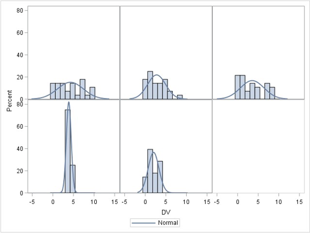
### Normality check for the whole samples
- Assume that the DV (Y) is distributed normally within each group for ANOVA
- ANOVA is **robust** to minor violations of normality
- So generally start with homogeneity, then assess normality
------------------------------------------------------------------------
### R function `shapiro.test()`
```{r}
#| eval: true
#| code-fold: true
#| results: hold
set.seed(123)  # For reproducibility
sample_normal_data <- rnorm(200, mean = 50, sd = 10)  # Generate normal data
sample_nonnormal_data <- sample(1:10, 200, replace = TRUE)  # Generate non-normal data

cat("Normality assumption holds:")
shapiro.test(sample_normal_data)
cat("Normality assumption does not hold:")
shapiro.test(sample_nonnormal_data)
```
------------------------------------------------------------------------
### R function `ks.test()`
```{r}
#| results: hold
# Perform Kolmogorov-Smirnov test against a normal distribution
cat("Normality assumption holds:")
ks.test(scale(sample_normal_data), "pnorm")
cat("Normality assumption does not hold:")
ks.test(scale(sample_nonnormal_data), "pnorm")
```
::: panel-tabset
### Exercise II
Perform Shapiro-Wilk and Kolmogorov-Smirnov for both datasets. Tell me which test works or does not work and why.
```{webr-r}
set.seed(2345)
normal_data <- rnorm(50, mean = 50, sd = 10) # normal data
nonnormal_data <- sample(1:10, 50, replace = TRUE) # non-normal
### Perform Shapiro-Wilk and Kolmogorov-Smirnov for both data
### Shapiro-Wilk
_____(normal_data)
_____(nonnormal_data)
### Kolmogorov-Smirnov
_____(____(normal_data, _____))
_____(____(nonnormal_data, _____))
```
### Answer
```{webr-r}
shapiro.test(normal_data)
shapiro.test(nonnormal_data)
ks.test(scale(normal_data), "pnorm")
ks.test(scale(nonnormal_data), "pnorm")
```
:::
-----------------------
### Normality check for each group
```{r}
#| code-fold: false
#| warning: false
# Generate three-group data with normal distributions
library(dplyr) # we need this package to group the data
set.seed(123)
group_data <- data.frame(
  group = rep(c("A", "B", "C"), each = 30),
  score = c(rnorm(30, mean = 50, sd = 10),  # Group A
            rnorm(30, mean = 55, sd = 12),  # Group B
            rnorm(30, mean = 48, sd = 9))   # Group C
)

# Run Shapiro-Wilk test for each group
group_data |>
  group_by(group) |>
  summarize(
    shapiro_p_value = shapiro.test(score)$p.value
  )
```
::: {.callout-tip collapse="true" title="R Tip: what does the pipe |> do?"}
- The [pipe]{.redcolor} `|>` takes whatever is on its **left** and passes it as the [first argument]{.bluecolor} of the function on its **right**. Read it out loud as the word ["then"]{.redcolor}.
| Written with the pipe | Same thing without it |
|-----------------------|-----------------------|
| `group_data |> head()` | `head(group_data)` |
| `group_data |> group_by(group)` | `group_by(group_data, group)` |
- So the code above says: *take `group_data`,* [then]{.redcolor} *split it by `group`,* [then]{.redcolor} *summarize each piece with a Shapiro-Wilk p-value.* Without the pipe you would have to nest the calls inside out, which reads backwards:
```{r}
#| eval: false
# Same result, harder to read -- start from the innermost call
summarize(group_by(group_data, group),
          shapiro_p_value = shapiro.test(score)$p.value)
```
- Notes:
- `|>` is the **native** pipe, built into R since version 4.1 — no package needed.
- You may also see `%>%`, the older **magrittr** pipe that comes with `dplyr`. For our purposes they behave the same.
- Keyboard shortcut in RStudio/Positron: [Ctrl/Cmd + Shift + M]{.bluecolor}.
- Put each step on its own line, ending the line with `|>`. R then knows the expression continues on the next line.
:::
**Interpretation of Normality Checking Results:**
- If all p-values > 0.05: All groups satisfy normality assumption - proceed with ANOVA
- If one group has p-value < 0.05 but others are normal:
- ANOVA is generally robust to minor normality violations, especially with equal sample sizes
- Consider the sample size: larger samples (n > 30) make ANOVA more robust
- Options: (1) Continue with ANOVA if violation is mild, (2) Apply data transformation (log, square root), or (3) Use non-parametric alternative (Kruskal-Wallis test)
- If multiple groups violate normality: Strong evidence against using ANOVA - consider transformations or non-parametric tests
--------
::: panel-tabset
### Exercise III
Perform Shapiro-Wilk for each group datasets. Tell me which group is not normal.
```{webr-r}
#| context: setup
set.seed(2345)
group_data2 <- data.frame(
group = rep(c("A", "B", "C"), each = 30),
score = c(round(rnorm(30, mean = 50, sd = 10), 2), # Group A
sample(seq(50, 100, .01), 30, replace = TRUE), # Group B
round(rnorm(30, mean = 48, sd = 9), 2)) # Group C
)
```
```{webr-r}
library(dplyr) # we need this package to group the data
head(group_data2) # check first 6 rows
### Perform Shapiro-Wilk for each group
group_data2 |>
______(______) |>
______(
shapiro_p_value = __________(________)$__________
)
```
### Answer
```{webr-r}
group_data2 |>
group_by(group) |>
summarize(
shapiro_p_value = shapiro.test(score)$p.value
)
```
:::
--------------------------------------------------------------------
## ANOVA Robustness
- **Robust to**:
- Minor normality violations (for large samples).
- Small HOV violations if group sizes are **equal**.
- **Not robust to**:
- **Independence violations**—ANOVA is invalid if data points are dependent.
- **Severe HOV violations**—Type I error rates become unreliable.
- The robustness of assumptions is something you should be careful about before/when you perform data collection. They are not something you can address after data collection has been finished.
------------------------------------------------------------------------
[Robustness to Violations of Normality Assumption]{.redcolor}
- ANOVA assumes that the residuals (errors) are normally distributed within each group.
- However, ANOVA is generally robust to violations of normality, particularly when **the sample size is large**.
- **Theoretical Justification**: This robustness is primarily due to the Central Limit Theorem (CLT), which states that, for sufficiently large sample sizes (typically $n≥30$ per group), the sampling distribution of the mean approaches normality, even if the underlying population distribution is non-normal.
- This means that unless the data are heavily skewed or have extreme outliers, ANOVA results remain valid and Type I error rates are not severely inflated.
------------------------------------------------------------------------
### Robustness to Violations of Homogeneity of Variance
- The homogeneity of variance (homoscedasticity) assumption states that all groups should have equal variances. ANOVA can tolerate moderate violations of this assumption, particularly when:
- **Sample sizes are equal (or nearly equal) across groups** – When groups have equal sample sizes, the F-test remains robust to variance heterogeneity because the pooled variance estimate remains balanced.
- **The degree of variance heterogeneity is not extreme** – If the largest group variance is no more than about four times the smallest variance, ANOVA results tend to remain accurate.
------------------------------------------------------------------------
### ANOVA: Lack of Robustness to Violations of Independence of Errors
- The assumption of independence of errors means that observations within and between groups must be uncorrelated. Violations of this assumption severely compromise ANOVA’s validity because:
- **Inflated Type I error rates** – If errors are correlated (e.g., due to clustering or repeated measures), standard errors are underestimated, leading to an increased likelihood of falsely rejecting the null hypothesis.
- **Biased parameter estimates** – When observations are not independent, the variance estimates do not accurately reflect the true variability in the data, distorting F-statistics and p-values.
- **Common sources of dependency** – Examples include nested data (e.g., students within schools), repeated measurements on the same subjects, or time-series data. In such cases, alternatives like mixed-effects models or generalized estimating equations (GEE) should be considered.
# Omnibus ANOVA Test
## Overview
- **What does it test?**
- Whether there is **at least one** significant difference among means.
- **Limitation**:
- Does **not** tell **which** groups are different.
- **Solution**:
- Conduct **post-hoc tests**.
## Individual Comparisons of Means
- If ANOVA is **significant**, follow-up tests identify **where** differences occur.
- **Types**:
- **Unplanned (post-hoc) comparisons**: Conducted **after** ANOVA (Ominibus ANOVA Test; Post-hoc Test).
- **Planned comparisons**: Defined **before** data collection.
## Planned vs. Unplanned Comparisons
- **Unplanned (post-hoc)**:
- **Data-driven**.
- Only performed **if ANOVA is significant**.
- **Planned**:
- Based on **theory**.
- Can be done **even if ANOVA is not significant**.
## Types of Unplanned Comparisons
- **Common post-hoc tests**:
1. **Tukey’s HSD**
2. **Family-Wise Error Rate** or Adjusted p-values
3. **Fisher’s LSD**
4. **Sidák correction**
------------------------------------------------------------------------
### Post-hoc test
[Tukey’s HSD]{.bluecolor}
- Controls for **Type I error** across multiple comparisons.
- Uses a **q-statistic** from a Tukey table.
- Preferred when **all pairs** need comparison.
```{r}
aov_result <- aov(score ~ group, group_data) # run the ANOVA model first
TukeyHSD(aov_result) # call TukeyHSD followed by the model to perform Tukey multiple comparisons
```
[Family-wise Error Rate (adjusted p-values)]{.bluecolor}
- Adjusts p-values to reduce Type I error
- Report adjusted p-values (typically larger that original p-values)
### Tukey Honest Significant Differences (HSD) Test
- **Purpose**: Conducts all possible pairwise comparisons between group means while controlling the family-wise error rate at the specified alpha level (typically 0.05).
- **Why it's needed**: Simple pairwise t-tests after a significant ANOVA inflate the Type I error rate. Tukey HSD adjusts for multiple comparisons to maintain the overall error rate.
- **How it works**: Creates confidence intervals for all pairwise mean differences using the studentized range distribution, which accounts for the number of groups being compared.
- **Interpretation**: If a confidence interval does not include zero, or if p adj < 0.05, the pair of groups differs significantly.
```{r}
#| eval: true
tukey_result <- TukeyHSD(aov_result)
print(tukey_result$group)
```
**Interpretation**: The Tukey HSD test provides pairwise comparisons between all groups while controlling for family-wise error rate. The output shows:
- **diff**: The difference in means between each pair of groups
- **lwr & upr**: The 95% confidence interval for the difference
- **p adj**: The adjusted p-value for multiple comparisons
Pairs with p adj < 0.05 indicate statistically significant differences between those groups.
------------------------------------------------------------------------
```{r}
#| eval: true
plot(tukey_result)
```
## Interpreting Results
### ANOVA Statistics
```
           Df Sum Sq Mean Sq F value   Pr(>F)
group        3  724.1  241.37   11.45 2.04e-05 ***
Residuals   36  759.2   21.09
---
Signif. codes:  0 '***' 0.001 '**' 0.01 '*' 0.05 '.' 0.1 ' ' 1
```
```{r}
#| eval: false
#| code-fold: true
library(dplyr)
data |>
  group_by(group) |>
  summarise(
    Mean = mean(score),
    SD = sd(score)
  )
```
- A one-way analysis of variance (ANOVA) was conducted to examine the effect of teaching method on students' test scores. The results indicated a statistically significant difference in test scores across the four groups, (F(3, 36) = 11.45, p < .001). Post-hoc comparisons using the Tukey HSD test revealed that the Interactive method (G3) (M = 28.06, SD = 3.33) resulted in significantly higher scores than the Traditional method (M = 18.17, SD = 4.47) with p < .001. However, no significant difference was found between G1 and the Control group (p = .99). These results suggest that certain teaching methods can significantly improve student performance compared to traditional approaches.
## ANOVA Example: Intervention and Verbal Acquisition
### Background
- Research Question: Does an intensive intervention improve students’ verbal acquisition scores?
- Study Design:
- 4 groups: Control, G1, G2, G3 (treatment levels).
- Outcome variable: Verbal acquisition score (average of three assessments).
- Hypotheses:
- $H_0$: No difference in verbal acquisition scores across groups.
- $H_A$: At least one group has a significantly different mean.
### Step 1: Generate Simulated Data in R
```{r}
#| warning: false
#| message: false
#| results: hold
# Load necessary libraries
library(tidyverse)

# Set seed for reproducibility
set.seed(123)

# Generate synthetic data for 4 groups
data <- tibble(
  group = rep(c("Control", "G1", "G2", "G3"), each = 30),
  verbal_score = c(
    rnorm(30, mean = 70, sd = 10),  # Control group
    rnorm(30, mean = 75, sd = 12),  # G1
    rnorm(30, mean = 80, sd = 10),  # G2
    rnorm(30, mean = 85, sd = 8)    # G3
  )
)

# View first few rows
head(data)
```
**Function explanations:**
- `library(tidyverse)`: Loads the tidyverse package collection, including dplyr, ggplot2, and tibble
- `set.seed(123)`: Sets the random number generator seed to ensure reproducible results across runs
- `tibble()`: Creates a modern data frame (tibble) with improved printing and subsetting behavior
- `rep(c("Control", "G1", "G2", "G3"), each = 30)`: Repeats each group label 30 times, creating 120 total observations (30 per group)
- `rnorm(30, mean = X, sd = Y)`: Generates 30 random numbers from a normal distribution with specified mean and standard deviation
- `c()`: Combines the four vectors of random numbers into a single vector of 120 values
- `head(data)`: Displays the first 6 rows of the dataset for preview
### Step 2: Summary Statistics
```{r}
# Summary statistics by group
data|>
  group_by(group)|>
  summarise(
    mean_score = mean(verbal_score),
    sd_score = sd(verbal_score),
    n = n()
  )
```
**Function explanations:**
- `group_by(group)`: Groups the data by the `group` variable, allowing subsequent operations to be performed separately for each group
- `summarise()`: Creates summary statistics for each group, collapsing the grouped data into summary values
- `mean(verbal_score)`: Calculates the arithmetic mean of verbal scores within each group
- `sd(verbal_score)`: Computes the standard deviation of verbal scores within each group
- `n()`: Counts the number of observations in each group
------------------------------------------------------------------------
```{r}
# Boxplot visualization
library(ggplot2)  # Load ggplot2 package for creating visualizations
ggplot(data, aes(x = group, y = verbal_score, fill = group)) +  # Create base plot with group on x-axis, scores on y-axis, fill by group
  geom_boxplot() +  # Add boxplot layer to show distribution of scores within each group
  theme_minimal() +  # Apply minimal theme for clean appearance
  labs(title = "Verbal Acquisition Scores Across Groups", y = "Score", x = "Group")  # Add descriptive labels
```
### Step 3: Check ANOVA Assumptions
### Assumption Check: Independence of residuals
```{r}
#| results: hold
#| warning: false
#| message: false
# Fit the ANOVA model
anova_model <- lm(verbal_score ~ group, data = data)

# Load the lmtest package
library(lmtest)

# Perform the Durbin-Watson test
dw_test_result <- dwtest(anova_model)

# View the test results
print(dw_test_result)
```
- Interpretation:
- In this example, the `DW` value is close to 2, and the p-value is greater than 0.05, indicating no significant autocorrelation in the residuals.
------------------------------------------------------------------------
### Assumption Check: Normality
```{r}
# Shapiro-Wilk normality test for each group
data |>
  group_by(group) |>
  summarise(
    shapiro_p = shapiro.test(verbal_score)$p.value
  )
```
- Interpretation:
- If $p>0.05$, normality assumption is not violated.
- If $p<0.05$, data deviates from normal distribution.
- Since the data meets the normality requirement and no outliers, we can use [Bartlett's or Levene's tests]{.redcolor} for HOV checking.
------------------------------------------------------------------------
- Alternative Check: Q-Q Plot
```{r}
ggplot(data, aes(sample = verbal_score)) +
  geom_qq() + geom_qq_line() +
  facet_wrap(~group) +
  theme_minimal() +
  labs(title = "Q-Q Plot for Normality Check")
```
------------------------------------------------------------------------
### Assumption Check: Homogeneity of Variance (HOV)
```{r}
#| results: hold
#| warning: false
library(car) # for leveneTest
library(onewaytests) # for bf.test
data$group <- as.factor(data$group)
car::leveneTest(verbal_score ~ group, data = data)
cat("-----------------------------\n")
bartlett.test(verbal_score ~ group, data = data)
cat("-----------------------------\n")
onewaytests::bf.test(verbal_score ~ group, data = data)
```
- Interpretation:
- If $p>0.05$, variance is homogeneous (ANOVA assumption met).
- If $p<0.05$, variance differs across groups (consider Welch’s ANOVA).
- It turns out our data does not violate the homogeneity of variance assumption.
### Step 4: Perform One-Way ANOVA
```{r}
anova_model <- aov(verbal_score ~ group, data = data)
summary(anova_model)
```
- Interpretation:
- If $p<0.05$, at least one group mean is significantly different.
- If $p>0.05$, fail to reject $H0$ (no significant differences).
### Step 5: Post-Hoc Tests (Tukey's HSD)
- After finding a significant ANOVA result, we perform Tukey's HSD test to identify which specific groups differ from each other.
- For example, we can compare:
- G1 vs Control
- G2 vs Control
- G3 vs Control
- G2 vs G1
- G3 vs G1
- G3 vs G2
```{r}
#| code-fold: false
# Tukey HSD post-hoc test
tukey_results <- TukeyHSD(anova_model)
round(tukey_results$group, 3)
```
- Interpretation:
- Identifies which groups differ.
- If $p<0.05$, the groups significantly differ.
- G1-Control
- G2-Control
- G3-Control
- G3-G1
------------------------------------------------------------------------
### Step 6: Family-wise Error Rate Control
- General Linear Hypothesis Tests: `glht` function in multcomp package allow us to perform family-wise error rate control (using `adjusted p-values`).
- Alternatively, we can use `TukeyHSD` to adjust p values to control inflated Type I error.
$$
Y = \beta_0G_0+\beta_1G_1 +\beta_2G_2 +\beta_3G_3
$$
- When $\{G_0, G_1, G_2, G_3\}$ = $\{0, 1, 0, 0\}$, $Y = \beta_1$, which is the group difference between G1 with the control group
- When $\{G_0, G_1, G_2, G_3\}$ = $\{0, 0, 1, 0\}$, $Y = \beta_2$, which is the group difference between G2 with the control group
- When $\{G_0, G_1, G_2, G_3\}$ = $\{0, -1, 1, 0\}$, $Y = \beta_2 - \beta_1$, which is the group difference between G2 with G1
```{r}
#| warning: false
#| message: false
#| results: hold
library(multcomp)
# install.packages("multcomp")
### set up multiple comparisons object for all-pair comparisons
# head(model.matrix(anova_model))
comprs <- rbind(
  "G1 - Ctrl" = c(0, 1, 0,  0),
  "G2 - Ctrl" = c(0, 0, 1,  0),
  "G3 - Ctrl" = c(0, 0, 0,  1),
  "G2 - G1" = c(0, -1, 1,  0),
  "G3 - G1" = c(0, -1, 0,  1),
  "G3 - G2" = c(0, 0, -1,  1)
)
cht <- glht(anova_model, linfct = comprs)
cht_fdr <- summary(cht, test = adjusted("fdr"))

# Wrap the console output into a reader-friendly table
fdr_table <- tibble(
  Comparison = names(cht_fdr$test$coefficients),
  Estimate   = round(as.numeric(cht_fdr$test$coefficients), 2),
  SE         = round(as.numeric(cht_fdr$test$sigma), 2),
  t          = round(as.numeric(cht_fdr$test$tstat), 2),
  p_value    = as.numeric(cht_fdr$test$pvalues)
) |>
  dplyr::mutate(
    Sig = dplyr::case_when(p_value < .001 ~ "***", p_value < .01 ~ "**",
                           p_value < .05  ~ "*",   TRUE ~ ""),
    `p (FDR)` = ifelse(p_value < .001, "< .001", sprintf("%.3f", p_value))
  ) |>
  dplyr::select(Comparison, Estimate, SE, t, `p (FDR)`, Sig)

knitr::kable(fdr_table, align = "lrrrrl",
             caption = "Pairwise comparisons with FDR-adjusted p-values")
```
- [Note]{.bluecolor}: `*` $p<.05$, `**` $p<.01$, `***` $p<.001$. `Estimate` is the mean difference; a positive value means the first group scored higher.
- All three interventions beat the control, and [G3 also beats G1]{.redcolor} — but G2 vs. G1 and G3 vs. G2 are not significant after FDR adjustment.
------------------------------------------------------------------------
### Side-by-Side comparison of two methods
::::: columns
::: {.column width="50%"}
#### TukeyHSD method
```{r}
#| eval: false
#| code-line-numbers: false
#| code-summary: "TukeyHSD method"
             diff    lwr    upr p adj
G1-Control  7.611  1.545 13.677 0.008 **
G2-Control 10.715  4.649 16.782 0.000 ***
G3-Control 14.720  8.654 20.786 0.000 ***
G2-G1       3.104 -2.962  9.170 0.543
G3-G1       7.109  1.042 13.175 0.015 *
G3-G2       4.005 -2.062 10.071 0.318
```
:::
::: {.column width="50%"}
#### FDR method
```{r}
#| eval: false
#| code-line-numbers: false
#| code-summary: "multcomp package"
               Estimate Std. Error t value Pr(>|t|)
G1 - Ctrl == 0    7.611      2.327   3.270  0.00283 **
G2 - Ctrl == 0   10.715      2.327   4.604 3.20e-05 ***
G3 - Ctrl == 0   14.720      2.327   6.325 2.94e-08 ***
G2 - G1 == 0      3.104      2.327   1.334  0.18487
G3 - G1 == 0      7.109      2.327   3.055  0.00419 **
G3 - G2 == 0      4.005      2.327   1.721  0.10555
```
:::
- The differences in p-value adjustment between the `TukeyHSD` method and the `multcomp` package stem from how each approach calculates and applies the multiple comparisons correction. Below is a detailed explanation of these differences.
:::::
### Comparison of Differences
| Feature | `TukeyHSD()` (Base R) | `multcomp::glht()` |
|----|----|----|
| **Distribution Used** | Studentized Range (q-distribution) | t-distribution |
| **Error Rate Control** | Strong FWER control | Flexible error control |
| **Simultaneous Confidence Intervals** | Yes | Typically not (depends on method used) |
| **Adjustment Method** | Tukey-Kramer adjustment | Single-step, Westfall, Holm, Bonferroni, etc. |
| **P-value Differences** | More conservative (larger p-values) | Slightly different due to t-distribution |
### Step 7: Reporting ANOVA Results
::: {.callout-note icon="false" title="Sample Write-Up — Results"}
1. We first examined three assumptions of ANOVA for our data as the preliminary analysis. According to the Durbin-Watson test, the Shapiro-Wilk normality test, and the Bartletts' test, the sample data meets all assumptions of the one-way ANOVA modeling.
2. A one-way ANOVA was then conducted to examine the effect of three intensive intervention methods (Control, G1, G2, G3) on verbal acquisition scores. There was a statistically significant difference between groups, $F(3,116)=14.33$, $p<.001$.
3. To further examine which intervention method is most effective, we performed Tukey's post-hoc comparisons. The results revealed that all three intervention methods have significantly higher scores than the control group (G1-Ctrl: p = .003; G2-Ctrl: p \< .001; G3-Ctrl: p \< .001). Among the three intervention methods, G3 seems to be the most effective. Specifically, G3 showed significantly higher scores than G1 (p = .004). However, no significant difference was found between G2 and G3 (p = .105).
:::
::: {.callout-tip icon="false" title="Sample Write-Up — Discussion"}
These findings suggest that higher intervention intensity improves verbal acquisition performance, which is consistent with prior literature \[xxxx/references\].
:::
# After-Class Exercise: Effect of Sleep Duration on Cognitive Performance
## Background
- Research Question:
- Does the amount of sleep affect cognitive performance on a standardized test?
- Study Design
- Independent variable: Sleep duration (3 groups: Short (≤5 hrs), Moderate (6-7 hrs), Long (≥8 hrs)).
- Dependent variable: Cognitive performance scores (measured as test scores out of 100).
---------------------------------------------
::: panel-tabset
### Exercise
```{webr-r}
#| context: setup
# Set seed for reproducibility
set.seed(42)
# Generate synthetic data for sleep study
sleep_data <- data.frame(
sleep_group = rep(c("Short", "Moderate", "Long"), each = 30),
cognitive_score = c(
rnorm(30, mean = 65, sd = 10), # Short sleep group (≤5 hrs)
rnorm(30, mean = 75, sd = 12), # Moderate sleep group (6-7 hrs)
rnorm(30, mean = 80, sd = 8) # Long sleep group (≥8 hrs)
)
)
```
```{webr-r}
# load packages you need
library(dplyr)
library(ggplot2)
library(lmtest)
library(car)
# View first few rows
head(sleep_data)
# Summary statistics by sleep group
sleep_data |>
group_by(sleep_group) |>
summarise(
_______
)
# Step 3: Check ANOVA Assumptions
# Indepdendence check: Perform the Durbin-Watson test
dw_test_result <- ____(____(_________, data = sleep_data))
# View the test results
print(dw_test_result)
# Normality check: Shapiro-Wilk normality test for each group
sleep_data |>
group_by(sleep_group) |>
summarise(
shapiro_p = ______(_______)$p.value
)
# HOV check: Levene's Test for homogeneity of variance
______(_______, data = sleep_data)
# Step 5: Perform One-Way ANOVA
anova_sleep <- ________(__________, data = sleep_data)
summary(anova_sleep)
# Step 6: Type I error control -- Tukey HSD post-hoc test
tukey_sleep <- TukeyHSD(_______)
tukey_sleep
```
### Answer
```{webr-r}
#| eval: false
#| echo: false
library(dplyr)
library(ggplot2)
library(lmtest)
library(car)
# View first few rows
head(sleep_data)
# Summary statistics by sleep group
sleep_data |>
group_by(sleep_group) |>
summarise(
mean_score = mean(cognitive_score),
sd_score = sd(cognitive_score),
n = n()
)
# Boxplot visualization
ggplot(sleep_data, aes(x = sleep_group, y = cognitive_score, fill = sleep_group)) +
geom_boxplot() +
theme_minimal() +
labs(title = "Cognitive Performance Across Sleep Groups", y = "Test Score", x = "Sleep Duration")
# Step 3: Check ANOVA Assumptions
# Indepdendence check: Perform the Durbin-Watson test
dw_test_result <- dwtest(aov(cognitive_score ~ sleep_group, data = sleep_data))
# View the test results
print(dw_test_result)
# Normality check: Shapiro-Wilk normality test for each group
sleep_data |>
group_by(sleep_group) |>
summarise(
shapiro_p = shapiro.test(cognitive_score)$p.value
)
ggplot(sleep_data, aes(sample = cognitive_score)) +
geom_qq() + geom_qq_line() +
facet_wrap(~sleep_group) +
theme_minimal() +
labs(title = "Q-Q Plot for Normality Check")
# HOV check: Levene's Test for homogeneity of variance
leveneTest(cognitive_score ~ sleep_group, data = sleep_data)
# Step 5: Perform One-Way ANOVA
anova_sleep <- aov(cognitive_score ~ sleep_group, data = sleep_data)
summary(anova_sleep)
# Step 6: Type I error control -- Tukey HSD post-hoc test
tukey_sleep <- TukeyHSD(anova_sleep)
tukey_sleep
```
::: heimu
- A one-way ANOVA was conducted to examine the effect of sleep duration on cognitive performance.
- There was a statistically significant difference in cognitive test scores across sleep groups, $F(2,87)=15.88$,$p<.001$.
- Tukey's post-hoc test revealed that participants in the Long sleep group (M=81.52, SD=6.27) performed significantly better than those in the Short sleep group (M=65.68, SD=12.55), p\<.01.
- These results suggest that inadequate sleep is associated with lower cognitive performance.
:::





