Hide the code
a = 1 + 1
b = a + 1
print(b)This file was created using Quarto, a type of document that allows you to review and execute all R code on this webpage.
To test a certain chunk of code, click the “copy” icon in the upper right corner of the chunk block (see screenshot below)
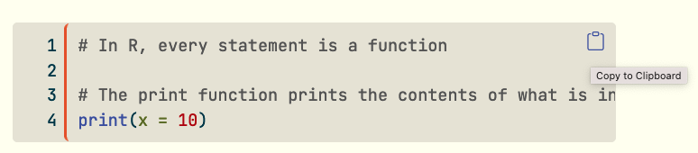
Try copying the following code
a = 1 + 1
b = a + 1
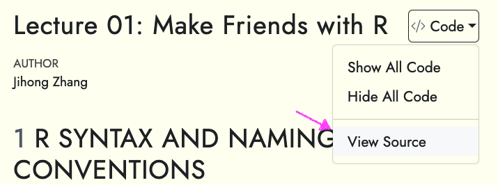
print(b)To review the whole file, click </> Code next to the title of this page. Find View Source and click the button. Then, you can paste the content into a newly created Quarto Document.
R is a powerful programming language and environment specifically designed for statistical computing and graphics. It’s free, open-source, and has a vast ecosystem of packages for data analysis, visualization, and machine learning.
R: The programming language and computing environment

RStudio: An integrated development environment (IDE) that makes R easier to use

# R comments begin with a # -- there are no multiline comments

# RStudio helps you build syntax
#   GREEN: Comments and character values in single or double quotes
#   BLUE: Functions and keywords
#   BLACK: Variable names and values

# You can use the tab key to complete object names, functions, and arguments

# R is case sensitive. That means R and r are two different things.

# Good naming conventions:
#   - Use descriptive names: my_data instead of x
#   - Use underscores or dots: my_data or my.data
#   - Avoid spaces and special characters (except . and _)
# - Don't start with numbers: 1data is invalid, data1 is valid# R has several basic data types:
# 1. Numeric (double) - decimal numbers
numeric_value <- 3.14
class(numeric_value)
# 2. Integer - whole numbers
integer_value <- 42L # The L suffix makes it an integer
class(integer_value)
# 3. Character (string) - text
character_value <- "Hello, R!"
class(character_value)
# 4. Logical (boolean) - TRUE/FALSE
logical_value <- TRUE
class(logical_value)
# 5. Complex - complex numbers
complex_value <- 3 + 4i
class(complex_value)
# Check the type of any object
typeof(numeric_value)
is.numeric(numeric_value)
is.character(character_value)# In R, every statement is a function
# The print function prints the contents of what is inside to the console
print(x = 10)
# The terms inside the function are called the arguments; here print takes x
# To find help with what the arguments are use:
?print
# Each function returns an object
print(x = 10)
# You can determine what type of object is returned by using the class function
class(print(x = 10))
# Function syntax: function_name(argument1, argument2, ...)
# Examples of common functions:
sqrt(16) # Square root
abs(-5) # Absolute value
round(3.14159, 2) # Round to 2 decimal places
length(c(1,2,3,4)) # Length of a vector
sum(c(1,2,3,4)) # Sum of values
mean(c(1,2,3,4)) # Mean of valuesVectors are the most basic data structure in R. They are one-dimensional arrays that can contain multiple elements of the same type (e.g., all numbers, all text, or all logical values).
# Use the c() function (combine) to create vectors
numeric_vector <- c(1, 2, 3, 4, 5)
character_vector <- c("apple", "banana", "cherry")
logical_vector <- c(TRUE, FALSE, TRUE)

# Display the vectors
numeric_vector
character_vector
logical_vector# Using the colon operator for simple sequences
sequence <- 1:10
sequence
# You can also create descending sequences
10:1# seq() gives you more control over sequences
# Create a sequence from 1 to 10, incrementing by 2
seq(from = 1, to = 10, by = 2)
# Create a sequence with exactly 5 equally-spaced values between 1 and 10
seq(1, 10, length.out = 5)# Repeat a single value multiple times
rep(5, times = 3)
# Repeat an entire vector multiple times
rep(c(1, 2), times = 3)
# Repeat each element multiple times before moving to the next
rep(c(1, 2), each = 3)# R performs operations element-wise on vectors
x <- c(1, 2, 3, 4, 5)
y <- c(10, 20, 30, 40, 50)
# Element-wise addition
x + y
# Element-wise multiplication
x * y
# Element-wise exponentiation
x^2
# You can also perform operations with a single value (vectorization)
x + 10
x * 2Factors are used for categorical variables in R. They store both the values and the levels (categories), which is essential for statistical analysis and plotting. R uses factors to understand categorical variables properly.
# Create a factor from a character vector
gender <- c("Male", "Female", "Male", "Female", "Male")
gender_factor <- factor(gender)
gender_factor

# Check the levels (categories)
levels(gender_factor)

# See how many observations in each category
table(gender_factor)# You can specify the order of levels explicitly
# This is useful when you want a specific order for plotting or analysis
education <- c("High School", "College", "Graduate", "High School")
education_factor <- factor(education,
levels = c("High School", "College", "Graduate"))
education_factor
# View the levels in the order you specified
levels(education_factor)# Use ordered = TRUE for ordinal data (categories with a meaningful order)
satisfaction <- c("Low", "Medium", "High", "Medium", "Low")
satisfaction_ordered <- factor(satisfaction,
levels = c("Low", "Medium", "High"),
ordered = TRUE)
satisfaction_ordered
# Notice the < signs indicating the order
print(satisfaction_ordered)# Get frequency counts
table(gender_factor)# Convert factor back to character
as.character(gender_factor)
# Convert to numeric (gives you the underlying level numbers, not always useful)
as.numeric(gender_factor)
# Be careful: converting numeric to factor
age_values <- c(25, 30, 35, 25, 40, 30)
age_factor <- factor(age_values)
age_factor # Notice it treats each unique number as a separate category# cut() is ideal for dividing continuous data into intervals
ages <- c(22, 25, 30, 35, 40, 45, 50, 55, 60, 65)
age_categories <- cut(ages,
breaks = c(0, 30, 50, 100), # Define the breakpoints
labels = c("Young", "Middle", "Senior"), # Label each interval
include.lowest = TRUE) # Include the lowest value in the first interval
age_categories
# Check the distribution
table(age_categories)# ifelse() gives you more control over custom conditions
ages <- c(22, 25, 30, 35, 40, 45, 50, 55, 60, 65)
age_groups_custom <- ifelse(ages < 30, "Young",
ifelse(ages < 50, "Middle", "Senior"))
# Convert to an ordered factor
age_groups_factor <- factor(age_groups_custom,
levels = c("Young", "Middle", "Senior"),
ordered = TRUE)
age_groups_factor
# View the distribution
table(age_groups_factor)
summary(age_groups_factor)Factors are essential because they:
# Each object can be saved into the R environment (the workspace here)
#   You can save the results of a function call to a variable of any name
MyObject = print(x = 10)
class(MyObject)

# You can view the objects you have saved in the Environment tab in RStudio
# Or type their name
MyObject

# There are literally thousands of types of objects in R (you can create them),
#   but for our course we will mostly be working with data frames (more later)

# The process of saving the results of a function to a variable is called
#   assignment. There are several ways you can assign function results to
#   variables:

# The equals sign takes the result from the right-hand side and assigns it to
#   the variable name on the left-hand side:
MyObject = print(x = 10)

# The <- (Alt "-" in RStudio) functions like the equals (right to left)
MyObject2 <- print(x = 10)

identical(MyObject, MyObject2)

# The -> assigns from left to right:
print(x = 10) -> MyObject3

identical(MyObject, MyObject2, MyObject3)

# Best practice: Use <- for assignment (more explicit)
# Use = only for function arguments# Lists can contain elements of different types
my_list <- list(
name = "John",
age = 30,
scores = c(85, 90, 78),
passed = TRUE
)
# Accessing list elements
my_list$name
my_list[["age"]]
my_list[[3]]
# Lists are very flexible and useful for complex data structures# Matrices are 2-dimensional arrays with the same data type
my_matrix <- matrix(1:12, nrow = 3, ncol = 4)
my_matrix
# Creating matrices from vectors
matrix(c(1,2,3,4,5,6), nrow = 2, ncol = 3)
# Matrix operations
matrix1 <- matrix(1:4, nrow = 2)
matrix2 <- matrix(5:8, nrow = 2)
matrix1 + matrix2
matrix1 * matrix2 # Element-wise multiplicationA data frame is an R object that stores data in a rectangular (table) format. Each column represents a variable and can be of different types (e.g., numeric, character, factor). Each row represents an observation or case.
We will start by importing data from a comma-separated values (csv) file.
We will use the read.csv() function. Here, the argument stringsAsFactors = FALSE prevents R from automatically converting character strings into factors (categorical variables), giving us more control over data types
We can use the here::here() function to create reliable file paths that work across different operating systems and project structures.
# You can also set the working directory using setwd().
# For example, to set it to your home folder:
# setwd("~")

getwd()  # Get current working directory
dir() # List files in current directory# The following might give an error if the file path is not correct from your current directory:
HeightsData = read.csv(file = "heights.csv",
stringsAsFactors = FALSE)
HeightsData# Note: Windows users need to use either forward slashes (/) or
# double backslashes (\\) in file paths. Single backslashes (\) don't work in R.
# Example: "C:/Users/name/file.csv" or "C:\\Users\\name\\file.csv"
# To view your data in RStudio, you can either:
# 1) Double-click the data frame in the Environment tab, or
# 2) Use the View() function
# View(HeightsData)
# You can access individual variables (columns) using the $ operator:
HeightsData$ID
# To read SPSS files, we need the foreign package.
# The foreign package comes pre-installed with R (no need to use install.packages()).
library(foreign)
# The read.spss() function imports an SPSS file.
# Setting to.data.frame = TRUE converts it to an R data frame (rather than a list)
WideData = read.spss(file = "wide.sav",
to.data.frame = TRUE)
WideData# Data frames are the most common data structure for statistical analysis
# They are like spreadsheets with rows (observations) and columns (variables)
# Basic data frame operations
dim(HeightsData) # Dimensions (rows, columns)
nrow(HeightsData) # Number of rows
ncol(HeightsData) # Number of columns
names(HeightsData) # Column names
str(HeightsData) # Structure of the data frame
head(HeightsData) # First 6 rows
tail(HeightsData) # Last 6 rows
summary(HeightsData) # Summary statistics
# Accessing data frame elements
HeightsData[1, 2] # Row 1, Column 2
HeightsData[1:5, ] # Rows 1-5, all columns
HeightsData[, "ID"] # All rows, column named "ID"
HeightsData$ID # Same as above (preferred method)
# Subsetting data frames
subset(HeightsData, HeightIN > 70)
HeightsData[HeightsData$HeightIN > 70, ]# The WideData and HeightsData have the same set of ID numbers.
# We can use the merge() function to merge them into a single data frame.
# Here, x is the name of the left-side data frame and y is the name of the
# right-side data frame. The arguments by.x and by.y specify the variable(s)
# by which we will merge:
AllData = merge(x = WideData, y = HeightsData, by.x = "ID", by.y = "ID")
AllData
## Method 2: Use dplyr method (the pipe operator |> can be typed using Ctrl+Shift+M on Windows or Cmd+Shift+M on Mac)
library(dplyr)
WideData |>
left_join(HeightsData, by = "ID")
# Different types of joins:
# left_join(): Keep all rows from left table
# right_join(): Keep all rows from right table
# inner_join(): Keep only rows that appear in both tables
# full_join(): Keep all rows from both tables# Sometimes, certain packages require repeated measures data to be in a long
# format (where each measurement is on a separate row rather than in separate columns).
library(dplyr) # contains variable selection
## Wrong Way (pivoting DV and Age separately creates unwanted combinations)
AllDataLong <- AllData |>
tidyr::pivot_longer(starts_with("DVTime"), names_to = "DV", values_to = "DV_Value") |>
tidyr::pivot_longer(starts_with("AgeTime"), names_to = "Age", values_to = "Age_Value")
OnePerson <- AllDataLong |>
filter(ID == "1")
OnePerson
## Correct Way (pivot both variables together, then separate and widen properly)
AllDataLong <- AllData |>
tidyr::pivot_longer(c(starts_with("DVTime"), starts_with("AgeTime"))) |>
tidyr::separate(name, into = c("Variable", "Time"), sep = "Time") |>
tidyr::pivot_wider(names_from = "Variable", values_from = "value") -> AllDataLong
OnePerson <- AllDataLong |>
filter(ID == "1")
OnePerson
# Understanding data reshaping:
# Wide format: Each time point has its own column
# Long format: Time points are in rows, with a time variableIn this exercise, you will practice reshaping repeated-measures data from wide format to long format using a dplyr pipeline (with tidyr functions).
id, time, dv, and age.dv by time as a verification step.# Load packages
library(dplyr)
library(tidyr)
# 1) Start from a small wide toy data set
toy_wide <- tibble::tribble(
~id, ~dv_time1, ~dv_time2, ~dv_time3, ~age_time1, ~age_time2, ~age_time3,
1, 10, 12, 15, 20, 21, 22,
2, 8, 11, 11, 19, 20, 21,
3, 14, 13, 16, 21, 22, 23
)
# 2) YOUR TURN: Convert to long using a single dplyr pipeline
# Goal columns: id, time (1/2/3), dv, age
# Hints:
# - Use pivot_longer() on both dv_ and age_ columns together
# - Separate the column name into variable (dv/age) and time (1/2/3)
# - Use pivot_wider() to spread variable back into dv and age columnstoy_long <- toy_wide |>
pivot_longer(
cols = c(starts_with("dv_"), starts_with("age_")),
names_to = "name",
values_to = "value"
) |>
separate(name, into = c("variable", "time"), sep = "_time") |>
pivot_wider(names_from = variable, values_from = value) |>
mutate(time = as.integer(time))
toy_long
toy_long |>
group_by(time) |>
summarize(mean_dv = mean(dv, na.rm = TRUE), .groups = "drop")# The dplyr package provides an intuitive set of functions for data manipulation
# Select columns
AllData |>
select(ID, starts_with("DV"))
# Filter rows
AllData |>
filter(ID < 5)
# Arrange rows
AllData |>
arrange(ID)
# Create new variables
AllData |>
mutate(
DV_avg = (DVTime1 + DVTime2 + DVTime3) / 3,
DV_range = DVTime3 - DVTime1
)
# Group and summarize
AllDataLong |>
group_by(Time) |>
summarize(
mean_DV = mean(DV, na.rm = TRUE),
sd_DV = sd(DV, na.rm = TRUE),
n = n()
)# The psych package provides convenient functions for computing descriptive statistics.
## If you haven't installed it yet, run: install.packages("psych")
library(psych)
# Use describe() to get comprehensive descriptive statistics for all variables:
DescriptivesWide = describe(AllData)
DescriptivesWide
DescriptivesLong = describe(AllDataLong)
DescriptivesLong
# Use describeBy() to compute descriptive statistics separately for each group:
DescriptivesLongID = describeBy(AllDataLong, group = AllDataLong$ID)
DescriptivesLongID
# Basic descriptive statistics without packages:
mean(AllDataLong$DV, na.rm = TRUE)
median(AllDataLong$DV, na.rm = TRUE)
sd(AllDataLong$DV, na.rm = TRUE)
var(AllDataLong$DV, na.rm = TRUE)
min(AllDataLong$DV, na.rm = TRUE)
max(AllDataLong$DV, na.rm = TRUE)
quantile(AllDataLong$DV, probs = c(0.25, 0.5, 0.75), na.rm = TRUE)# You can transform data by creating new variables.
AllDataLong$AgeC = AllDataLong$Age - mean(AllDataLong$Age)
# You can also use functions to create new variables. Here we create new terms
# using the function for significant digits:
AllDataLong$AgeYear = signif(x = AllDataLong$Age, digits = 2)
AllDataLong$AgeDecade = signif(x = AllDataLong$Age, digits = 1)
head(AllDataLong)
# Common data transformations:
# Centering: subtract mean
# Standardizing: (x - mean) / sd
# Log transformation: log(x)
# Square root: sqrt(x)
# Recoding: ifelse(condition, value_if_true, value_if_false)
# Example: Create standardized variables
AllDataLong$DV_z <- scale(AllDataLong$DV)
AllDataLong$Age_z <- scale(AllDataLong$Age)# R has excellent plotting capabilities
# Base R plotting
hist(AllDataLong$DV, main = "Distribution of DV", xlab = "DV Values")
boxplot(DV ~ Time, data = AllDataLong, main = "DV by Time")
plot(AllDataLong$Age, AllDataLong$DV, main = "DV vs Age")
# Using ggplot2 (more modern and flexible)
# If you have not install the package yet, type in install.packages("ggplot2")
library(ggplot2)
# Histogram
ggplot(AllDataLong, aes(x = DV)) +
geom_histogram(bins = 30) +
labs(title = "Distribution of DV", x = "DV Values", y = "Count")
# Boxplot
ggplot(AllDataLong, aes(x = Time, y = DV)) +
geom_boxplot() +
labs(title = "DV by Time")
# Scatter plot
ggplot(AllDataLong, aes(x = Age, y = DV)) +
geom_point() +
geom_smooth(method = "lm") +
labs(title = "DV vs Age")hw0_feedback <- read.csv(here::here("teaching/2025-01-13-Experiment-Design/Lecture01", "hw0_feedback.csv"))
table(hw0_feedback$Feedback)# Conditional statements (if-else)
x <- 10
if (x > 5) {
print("x is greater than 5")
} else {
print("x is less than or equal to 5")
}
## Alternative method using ifelse() function (vectorized)
ifelse(x > 5,
print("x is greater than 5"),
print("x is less than or equal to 5"))
# For loops (repeat code a specific number of times)
for (i in 1:5) {
print(paste("Iteration", i))
}
# While loops (repeat code while a condition is TRUE)
i <- 1
while (i <= 5) {
print(paste("While iteration", i))
i <- i + 1
}
# Apply functions (more efficient and "R-like" than explicit loops)
numbers <- 1:10
sapply(numbers, function(x) x^2) # Returns a vector
lapply(numbers, function(x) x^2) # Returns a list# R uses NA (Not Available) to represent missing data
# Check for missing values in a variable
is.na(AllDataLong$DV) # Returns TRUE/FALSE for each value
sum(is.na(AllDataLong$DV)) # Count the number of missing values
complete.cases(AllDataLong) # Check which rows have no missing data
# Remove rows that contain any missing data
AllDataLong_complete <- na.omit(AllDataLong)
# Alternative method (same result):
AllDataLong_complete <- AllDataLong[complete.cases(AllDataLong), ]
# Replace missing values with the mean (simple imputation)
AllDataLong$DV_imputed <- ifelse(is.na(AllDataLong$DV),
mean(AllDataLong$DV, na.rm = TRUE),
AllDataLong$DV)# 1. Always use meaningful variable names
# 2. Comment your code
# 3. Use consistent formatting
# 4. Check your data after importing
# 5. Save your work regularly
# 6. Use version control (Git)
# 7. Write reproducible code
# 8. Use packages for common tasks
# 9. Learn to use help documentation
# 10. Practice regularly!
# Useful keyboard shortcuts in RStudio:
# Ctrl+Enter (Cmd+Enter on Mac): Run the current line or selected code
# Ctrl+Shift+Enter (Cmd+Shift+Enter on Mac): Run the entire script
# Ctrl+Shift+M (Cmd+Shift+M on Mac): Insert the pipe operator |>
# Ctrl+Shift+C (Cmd+Shift+C on Mac): Comment or uncomment selected lines
# Ctrl+Shift+R (Cmd+Shift+R on Mac): Insert a code section header# R has excellent help documentation
?mean # Help for a function
??"regression" # Search for functions containing "regression"
help(mean) # Same as ?mean
example(mean) # Run examples for a function
# Online resources:
# - R Documentation: https://www.rdocumentation.org/
# - Stack Overflow: https://stackoverflow.com/questions/tagged/r
# - R-bloggers: https://www.r-bloggers.com/
# - RStudio Community: https://community.rstudio.com/
# Installing and loading packages
install.packages("package_name") # Install once
library(package_name) # Load each session
require(package_name) # Alternative to library()