---
title: "Lecture 10"
subtitle: "Generalized Measurement Models: Modeling Observed Polytomous Data"
author: "Jihong Zhang"
institute: "Educational Statistics and Research Methods"
title-slide-attributes:
data-background-image: ../Images/title_image.png
data-background-size: contain
execute:
echo: false
eval: false
format:
html:
code-tools: true
code-line-numbers: false
code-fold: true
code-summary: 'Click here to see R code'
number-offset: 1
fig.width: 10
fig-align: center
message: false
revealjs:
output-file: slides-index.html
logo: ../Images/UA_Logo_Horizontal.png
incremental: false # choose "false "if want to show all together
transition: slide
background-transition: fade
theme: [simple, ../pp.scss]
footer: <https://jihongzhang.org/posts/2024-01-12-syllabus-adv-multivariate-esrm-6553>
scrollable: true
slide-number: true
chalkboard: true
number-sections: false
code-line-numbers: true
code-annotations: below
code-copy: true
code-summary: ''
highlight-style: arrow
view: 'scroll' # Activate the scroll view
scrollProgress: true # Force the scrollbar to remain visible
mermaid:
theme: neutral
#bibliography: references.bib
---
## Previous Class
1. Dive deep into factor scoring
2. Show how different initial values affect Bayesian model estimation
3. Show how parameterization differs for standardized latent variables vs. marker item scale identification
## Today's Lecture Objectives
1. Show how to estimate unidimensional latent variable models with polytomous data
- Also know as [Polytomous]{.underline} I[tem response theory]{.underline} (IRT) or [Item factor analysis]{.underline} (IFA)
2. Distributions appropriate for polytomous (discrete; data with lower/upper limits)
## Example Data: Conspiracy Theories
- Today's example is from a bootstrap resample of 177 undergraduate students at a large state university in the Midwest.
- The survey was a measure of 10 questions about their beliefs in various conspiracy theories that were being passed around the internet in the early 2010s
- All item responses were on a 5-point Likert scale with:
1. Strong Disagree $\rightarrow$ 0
2. Disagree $\rightarrow$ 0
3. Neither Agree nor Disagree $\rightarrow$ 0
4. Agree $\rightarrow$ 1
5. Strongly Agree $\rightarrow$ 1
- The purpose of this survey was to study individual beliefs regarding conspiracies.
- Our purpose in using this instrument is to provide a context that we all may find relevant as many of these conspiracies are still prevalent.
## From Previous Lectures: CFA (Normal Outcomes)
For comparisons today, we will be using the model where we assumed each outcome was (conditionally) normally distributed:
For an item $i$ the model is:
$$
Y_{pi}=\mu_i+\lambda_i\theta_p+e_{pi}\\
e_{pi}\sim N(0,\psi_i^2)
$$
Recall that this assumption wasn't good one as the type of data (discrete, bounded, some multimodality) did not match the normal distribution assumption.
## Polytomous Data Characteristics
As we have done with each observed variable, we must decide which distribution to use
- To do this, we need to map the characteristics of our data on to distributions that share those characteristics
Our observed data:
- Discrete responses
- Small set of known categories: 1,2,3,4,5
- Some observed item responses may be multimodal
## Discrete Data Distributions
[Stan](https://mc-stan.org/docs/functions-reference/bounded_discrete_distributions.html) has a list of distributions for bounded discrete data
1. Binomial distribution
- Pro: Easy to use / code
- Con: Unimodal distribution
2. Beta-binomial distribution
- Not often used in psychometrics (but could be)
- Generalizes binomial distribution to have different probability for each trial
3. Hypergeometric distribution
- Not often used in psychometrics
4. Categorical distribution (sometimes called multinomial)
- Most frequently used
- Base distribution for graded response, partial credit, and nominal response models
5. Discrete range distribution (sometimes called uniform)
- Not useful–doesn't have much information about latent variables
# Binomial Distribution Models
## Binomial Distribution Models
The binomial distribution is one of the easiest to use for polytomous items
- However, it assumes the distribution of responses are unimodal
Binomial probability mass function (i.e., pdf):
$$
P(Y=y)=\begin{pmatrix}n\\y\end{pmatrix}p^y(1-p)^{(n-y)}
$$
Parameters:
- n - "number of trials" (range: $n \in \{0, 1, \dots\}$)
- y - "number of successes" out of $n$ "trials" (range: $y\in\{0,1,\dots,n\}$)
- p - "probability of success" (range: \[0, 1\])
- Mean: $np$
- Variance: $np(1-p)$
## Probability Mass Function
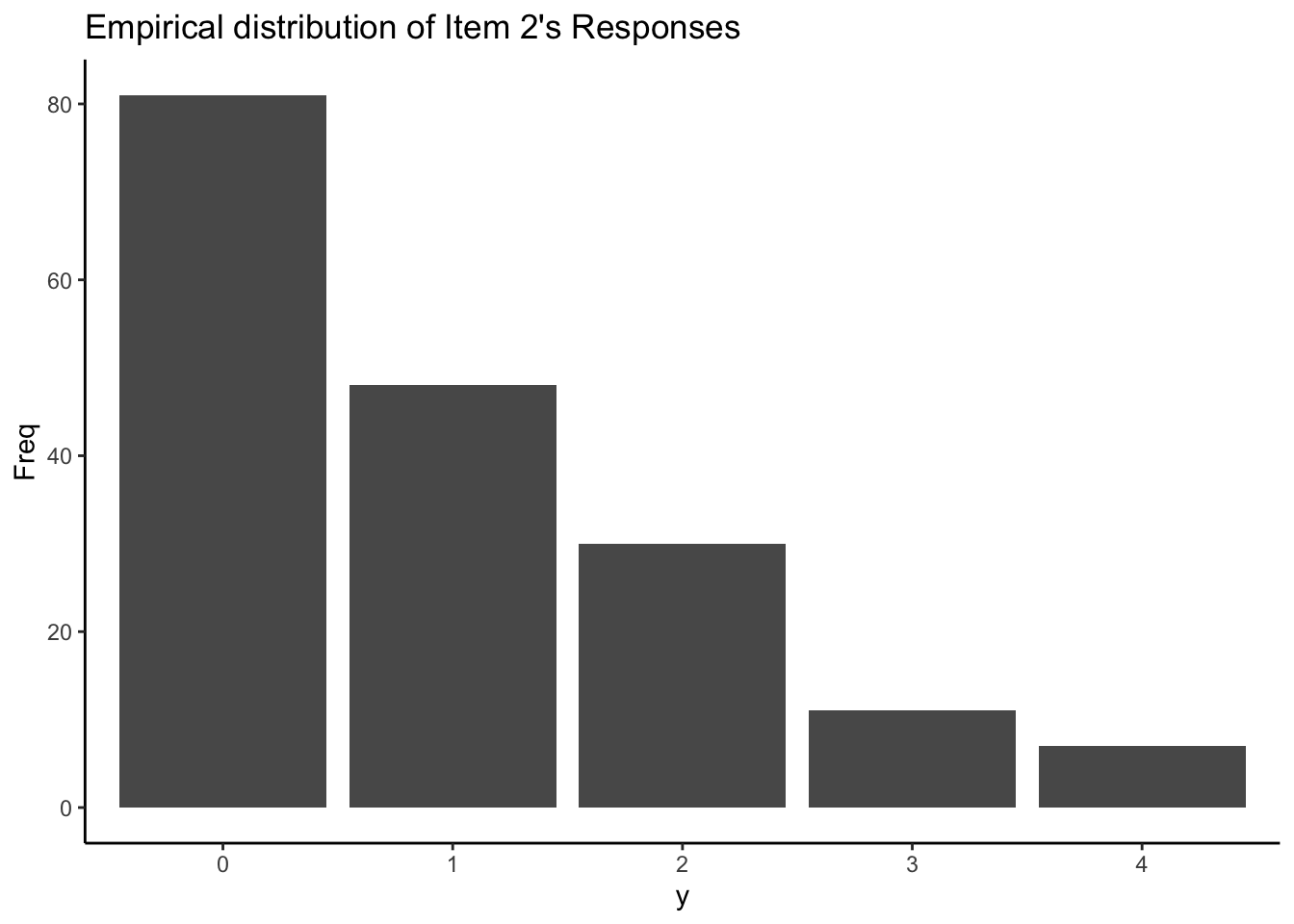
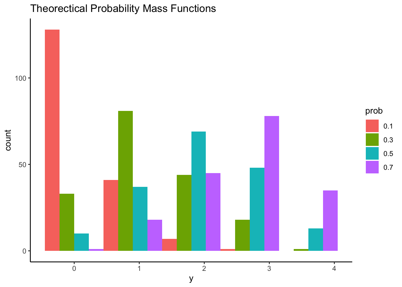
Fixing `n = 4` and probability of "brief in conspiracy theory" for each item `p = {.1, .3, .5, .7}` , we can know probability mass function across each item response from 0 to 4.
Question: which shape of distribution matches our data's empirical distribution most?
::: columns
::: {.column width="50%"}
```{r}
#| eval: true
library(tidyverse)
library(kableExtra)
library(here)
library(blavaan)
self_color <- c("#DB7093", "#AFEEEE", "#3CB371", "#9370DB", "#FFD700")
root_dir <- "teaching/2024-01-12-syllabus-adv-multivariate-esrm-6553/Lecture07/Code"
current_dir <- "teaching/2024-01-12-syllabus-adv-multivariate-esrm-6553/Lecture10/Code"
save_dir <- "~/Library/CloudStorage/OneDrive-Personal/2024_Spring/ESRM6553 - Advanced Multivariate Modeling/Lecture10"
dat <- read.csv(here(root_dir, 'conspiracies.csv'))
itemResp <- dat[,1:10]
colnames(itemResp) <- paste0('item', 1:10)
conspiracyItems = itemResp
as.data.frame(table(itemResp[,2]-1)) |>
ggplot() +
geom_col(aes(x = Var1, y = Freq)) +
labs(x = "y", title = "Empirical distribution of Item 2's Responses") +
theme_classic()
```
:::
::: {.column width="50%"}
```{r}
#| eval: true
set.seed(1234)
Reduce(rbind, lapply(c(.1, .3, .5, .7), \(x) data.frame(P = rbinom(n = 177, prob = x, size = 4), prob = x))) |>
mutate(prob = factor(prob, levels = c(.1, .3, .5, .7))) |>
ggplot() +
geom_histogram(aes(x = P, fill = prob), position = position_dodge(), binwidth = .9) +
labs(x = "y", title = "Theorectical Probability Mass Functions") +
theme_classic()
```
:::
:::
## Adapting the Binomial for Item Response Models
Although it doesn't seem like our items fit with a binomial, we can actually use this distribution
- Item response: number of successes $y_i$
- Needed: recode data so that lowest category is 0 (subtract one from each item)
- Highest (recoded) item response: number of trials $n$
- For all out items, once recoded, $n_i = 4$
- Then, use a link function to model each item's $p_i$ as a function of the latent trait:
$$
P(Y_i=y_i)=\begin{pmatrix}4\\y_i\end{pmatrix}p^{y_i}(1-p)^{(4-y_i)}
$$
where probability of success of item $i$ for individual $p$ is as:
$$
p_{pi}=\frac{\text{exp}(\mu_i+\lambda_i\theta_p)}{1+\text{exp}(\mu_i+\lambda_i\theta_p)}
$$
------------------------------------------------------------------------
Note:
- Shown with a logit link function (but could be any link)
- Shown in slope/intercept form (but could be distrimination/difficulty for unidimensional items)
- Could also include asymptote parameters ($c_i$ or $d_i$)
## Binomial Item Response Model
The item response model, put into the PDF of the binomial is then:
$$
P(Y_{pi}|\theta_p)=\begin{pmatrix}n_i\\Y_{pi}\end{pmatrix}(\frac{\text{exp}(\mu_i+\lambda_i\theta_p)}{1+\text{exp}(\mu_i+\lambda_i\theta_p)})^{y_{pi}}(1-\frac{\text{exp}(\mu_i+\lambda_i\theta_p)}{1+\text{exp}(\mu_i+\lambda_i\theta_p)})^{4-y_{pi}}
$$
Further, we can use the same priors as before on each of our item parameters
- $\mu_i$: Normal Prior $N(0, 100)$
- $\lambda_i$: Normal prior $N(0, 100)$
Likewise, we can identify the scale of the latent variable as before, too:
- $\theta_p \sim N(0,1)$
## `model{}` for the Binomial Model in Stan
```{stan, output.var='display'}
#| echo: true
model {
  lambda ~ multi_normal(meanLambda, covLambda); // Prior for item discrimination/factor loadings
  mu ~ multi_normal(meanMu, covMu);             // Prior for item intercepts
  theta ~ normal(0, 1);                         // Prior for latent variable (with mean/sd specified)
  for (item in 1:nItems){
    Y[item] ~ binomial(maxItem[item], inv_logit(mu[item] + lambda[item]*theta));
  }
}
```
Here, the binomial [item response function]{.underline} has two arguments:
- The **first** part: (`maxItem[Item]`) is the number of "trials" $n_i$ (here, our maximum score minus one – 4)
- The **second** part: (`inv_logit(mu[item] + lambda[item]*theta)`) is the probability from our model ($p_i$)
The data `Y[item]` must be:
- Type: integer
- Range: 0 through `maxItem[item]`
## `parameters{}` for the Binomial Model in Stan
```{stan, output.var='display'}
#| echo: true
parameters{
  vector[nObs] theta;                // the latent variables (one for each person)
  vector[nItems] mu;                 // the item intercepts (one for each item)
  vector[nItems] lambda;             // the factor loadings/item discriminations (one for each item)
}
```
No changes from any of our previous slope/intercept models
## `data{}` for the Binomial Model in Stan
```{stan, output.var='display'}
#| echo: true
data {
  int<lower=0> nObs;                     // number of observations
  int<lower=0> nItems;                   // number of items
  array[nItems] int<lower=0> maxItem;    // maximum value of Item (should be 4 for 5-point Likert)

  array[nItems, nObs] int<lower=0>  Y;   // item responses in an array

  vector[nItems] meanMu;                 // prior mean vector for intercept parameters
  matrix[nItems, nItems] covMu;          // prior covariance matrix for intercept parameters

  vector[nItems] meanLambda;             // prior mean vector for discrimination parameters
  matrix[nItems, nItems] covLambda;      // prior covariance matrix for discrimination parameters
}
```
Note:
- Need to supply `maxItem` (maximum score minus one for each item)
- The data are the same (integer) as in the binary/dichotomous item syntax
## Preparing Data for Stan
```{r}
#| echo: true
#| eval: true
# note: data must start at zero
conspiracyItemsBinomial = conspiracyItems
for (item in 1:ncol(conspiracyItemsBinomial)){
  conspiracyItemsBinomial[, item] = conspiracyItemsBinomial[, item] - 1
}

# check first item
table(conspiracyItemsBinomial[,1])
```
```{r}
#| echo: true
#| eval: true
# determine maximum value for each item
maxItem = apply(X = conspiracyItemsBinomial,
                MARGIN = 2,
                FUN = max)
maxItem
```
------------------------------------------------------------------------
### R Data List for Binomial Model
```{r}
#| echo: true
### Prepare data list -----------------------------
# data dimensions
nObs = nrow(conspiracyItems)
nItems = ncol(conspiracyItems)

# item intercept hyperparameters
muMeanHyperParameter = 0
muMeanVecHP = rep(muMeanHyperParameter, nItems)

muVarianceHyperParameter = 1000
muCovarianceMatrixHP = diag(x = muVarianceHyperParameter, nrow = nItems)

# item discrimination/factor loading hyperparameters
lambdaMeanHyperParameter = 0
lambdaMeanVecHP = rep(lambdaMeanHyperParameter, nItems)

lambdaVarianceHyperParameter = 1000
lambdaCovarianceMatrixHP = diag(x = lambdaVarianceHyperParameter, nrow = nItems)


modelBinomial_data = list(
  nObs = nObs,
  nItems = nItems,
  maxItem = maxItem,
  Y = t(conspiracyItemsBinomial),
  meanMu = muMeanVecHP,
  covMu = muCovarianceMatrixHP,
  meanLambda = lambdaMeanVecHP,
  covLambda = lambdaCovarianceMatrixHP
)
```
## Binomial Model Stan Call
```{r}
#| echo: true
modelBinomial_samples = modelBinomial_stan$sample(
  data = modelBinomial_data,
  seed = 12112022,
  chains = 4,
  parallel_chains = 4,
  iter_warmup = 5000,
  iter_sampling = 5000,
  init = function() list(lambda=rnorm(nItems, mean=5, sd=1))
)
```
1. Seed as 12112022
2. Number of Markov Chains as 4
3. Warmup Iterations as 5000
4. Sampling Iterations as 5000
5. Initial values of $\lambda$s as $N(5, 1)$
## Binomial Model Results
```{r}
#| echo: false
#| eval: true
modelBinomial_samples <- readRDS(here(save_dir, "modelBinomial_samples.RDS"))
```
```{r}
#| echo: true
#| eval: true
# checking convergence
max(modelBinomial_samples$summary(.cores = 4)$rhat, na.rm = TRUE)
```
```{r}
#| echo: true
#| eval: true
# item parameter results
print(modelBinomial_samples$summary(variables = c("mu", "lambda"), .cores = 4) ,n=Inf)
```
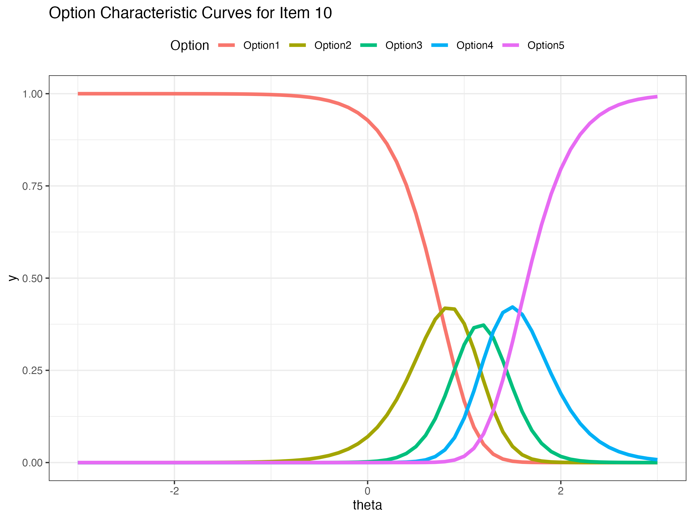
## Option Characteristic Curves
Expected probability of certain response across a range of latent variable $\theta$
{fig-align="center"}
## ICC for Item 10: The expected scores with latent variable
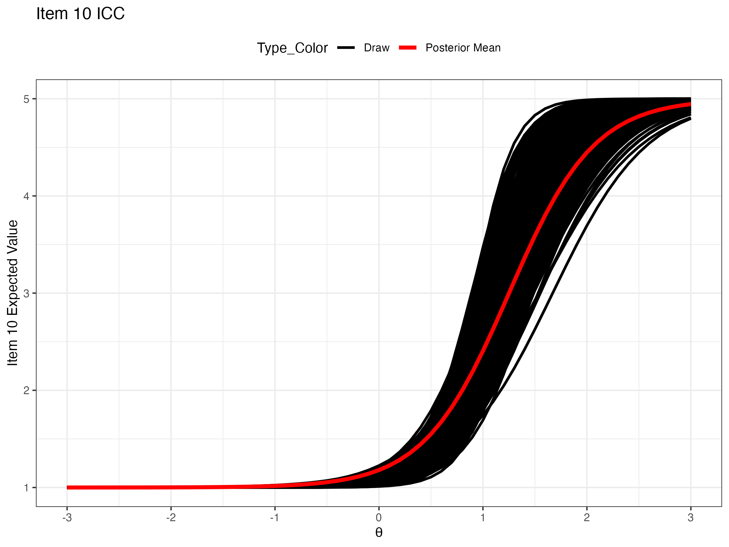{fig-align="center"}
## ICC for all items: which items have high expected score given theta
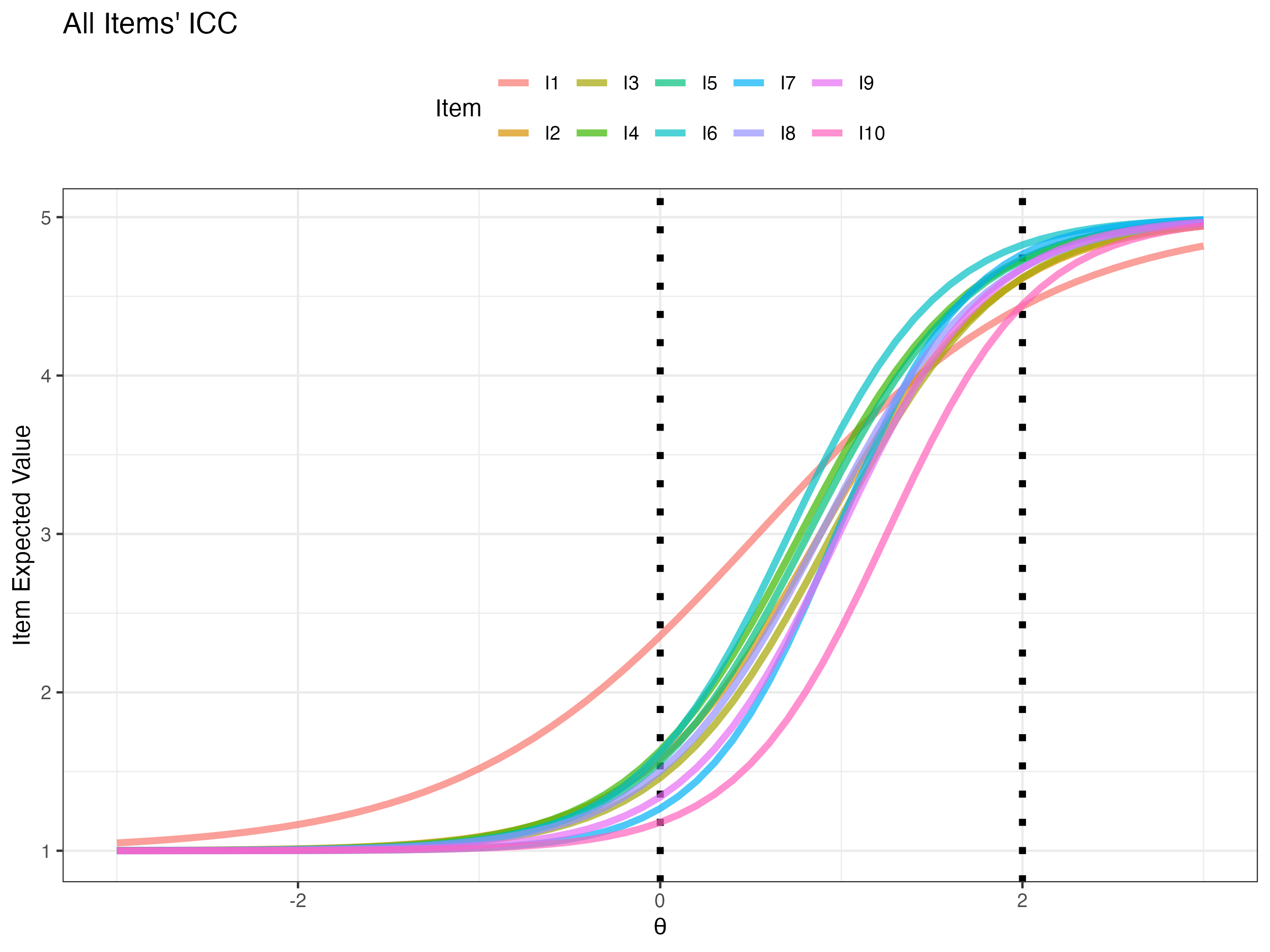{fig-align="center"}
## Investigate Latent Variable Estimates
Compare factors scores of Binomial model to 2PL-IRT
{fig-align="center"}
## Comparing EAP Estimates to Sum Scores
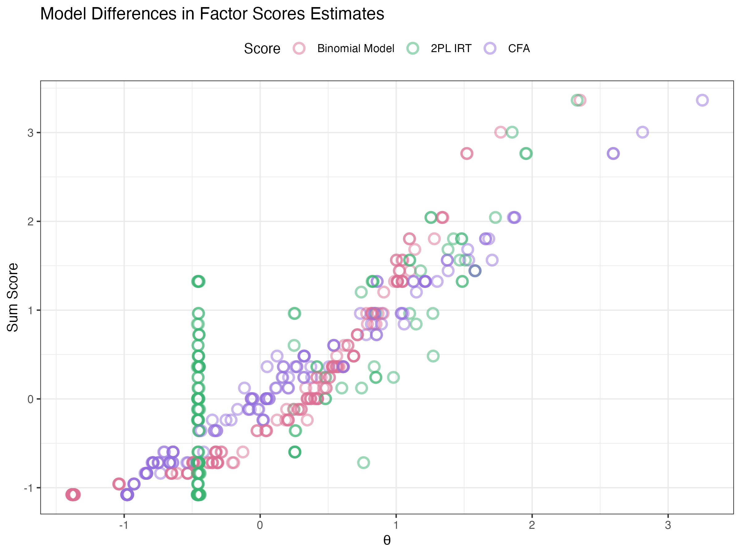{fig-align="center"}
# Categorical / Multinomial Distribution Models
## Multinomial Distribution Models
Although the binomial distribution is easy, it may not fit our data well
- Instead, we can use the categorical distribution, with following PMF:
$$
P(Y=y)=\frac{n!}{y_i!\dots y_C!}p_1^{y_1}\dots p_C^{y_C}
$$
Here,
- $n$: number of "trials"
- $y_c$: number of events in each of $c$ categories (c $\in \{1, \cdots, C\}$; $\Sigma_cy_c = n$)
- $p_c$: probability of observing an event in category $c$
## Graded Response Model (GRM)
GRM is one of the most popular model for ordered categorical response
$$
P(Y_{ic}|\theta) = 1 - P^*(Y_{i1}|\theta) \ \ \text{if}\ c=1\\
P(Y_{ic}|\theta) = P^*(Y_{i,c-1}|\theta)-P^*(Y_{i,c}|\theta) \ \ \text{if}\ 1<c<C\\
P(Y_{ic}|\theta) = P^*(Y_{i,C-1}|\theta) \ \ \text{if}\ c=C_i\\
$$where probability of response larger than $c$:
$$
P^*(Y_{i,c}|\theta) = P(Y_{i,c}>c|\theta)=\frac{\text{exp}(\mu_{ic}+\lambda_u\theta_p)}{1+\text{exp}(\mu_{ic}+\lambda_u\theta_p)}
$$
With:
- $C_i-1$ has ordered intercept intercepts: $\mu_i > \mu_2 > \cdots > \mu_{C_i-1}$
## `model{}` for GRM in Stan
```{stan, output.var='display'}
#| echo: true
model {

  lambda ~ multi_normal(meanLambda, covLambda); // Prior for item discrimination/factor loadings
  theta ~ normal(0, 1);                         // Prior for latent variable (with mean/sd specified)

  for (item in 1:nItems){
    thr[item] ~ multi_normal(meanThr[item], covThr[item]);             // Prior for item intercepts
    Y[item] ~ ordered_logistic(lambda[item]*theta, thr[item]);
  }

}
```
- `ordered_logistic` is the built-in Stan function for ordered categorical outcomes
- Two arguments neeeded for the function
- `lambda[item]*theta` is the muliplications
- `thr[item]` is the thresholds for the item, which is negative values of item intercept
- The function expects the response of Y starts from 1
## `parameters{}` for GRM in Stan
```{stan, output.var='display'}
#| echo: true
parameters {
  vector[nObs] theta;                // the latent variables (one for each person)
  array[nItems] ordered[maxCategory-1] thr; // the item thresholds (one for each item category minus one)
  vector[nItems] lambda;             // the factor loadings/item discriminations (one for each item)
}
```
Note that we need to declare threshould as: `ordered[maxCategory-1]` so that
$$
\tau_{i1} < \tau_{i2} <\cdots < \tau_{iC-1}
$$
## `generated quantities{}` for GRM in Stan
```{stan, output.var='display'}
#| echo: true
generated quantities{
  array[nItems] vector[maxCategory-1] mu;
  for (item in 1:nItems){
    mu[item] = -1*thr[item];
  }
}
```
Convert threshold back into item intercept
## `data{}` for GRM in Stan
```{stan, output.var='display'}
#| echo: true
data {
  int<lower=0> nObs;                            // number of observations
  int<lower=0> nItems;                          // number of items
  int<lower=0> maxCategory;

  array[nItems, nObs] int<lower=1, upper=5>  Y; // item responses in an array

  array[nItems] vector[maxCategory-1] meanThr;   // prior mean vector for intercept parameters
  array[nItems] matrix[maxCategory-1, maxCategory-1] covThr;      // prior covariance matrix for intercept parameters

  vector[nItems] meanLambda;         // prior mean vector for discrimination parameters
  matrix[nItems, nItems] covLambda;  // prior covariance matrix for discrimination parameters
}
```
Note that the input for the prior mean/covariance matrix for threshold parameters is now an array (one mean vector and covariance matrix per item)
## Prepare Data for GRM
To match the array for input for the threshold hyperparameter matrices, a little data manipulation is needed
```{r}
#| echo: true
# item threshold hyperparameters
thrMeanHyperParameter = 0
thrMeanVecHP = rep(thrMeanHyperParameter, maxCategory-1)
thrMeanMatrix = NULL
for (item in 1:nItems){
  thrMeanMatrix = rbind(thrMeanMatrix, thrMeanVecHP)
}

thrVarianceHyperParameter = 1000
thrCovarianceMatrixHP = diag(x = thrVarianceHyperParameter, nrow = maxCategory-1)
thrCovArray = array(data = 0, dim = c(nItems, maxCategory-1, maxCategory-1))
for (item in 1:nItems){
  thrCovArray[item, , ] = diag(x = thrVarianceHyperParameter, nrow = maxCategory-1)
}
```
R array matches Stan's array type
## GRM Results
```{r}
#| eval: true
modelOrderedLogit_samples <- readRDS(here(save_dir, "modelOrderedLogit_samples.RDS"))
```
```{r}
#| eval: true
#| echo: true
# checking convergence
max(modelOrderedLogit_samples$summary(.cores = 5)$rhat, na.rm = TRUE)
# item parameter results
print(modelOrderedLogit_samples$summary(variables = c("lambda", "mu"), .cores = 5) ,n=Inf)
```
## Option Characteristics Curve
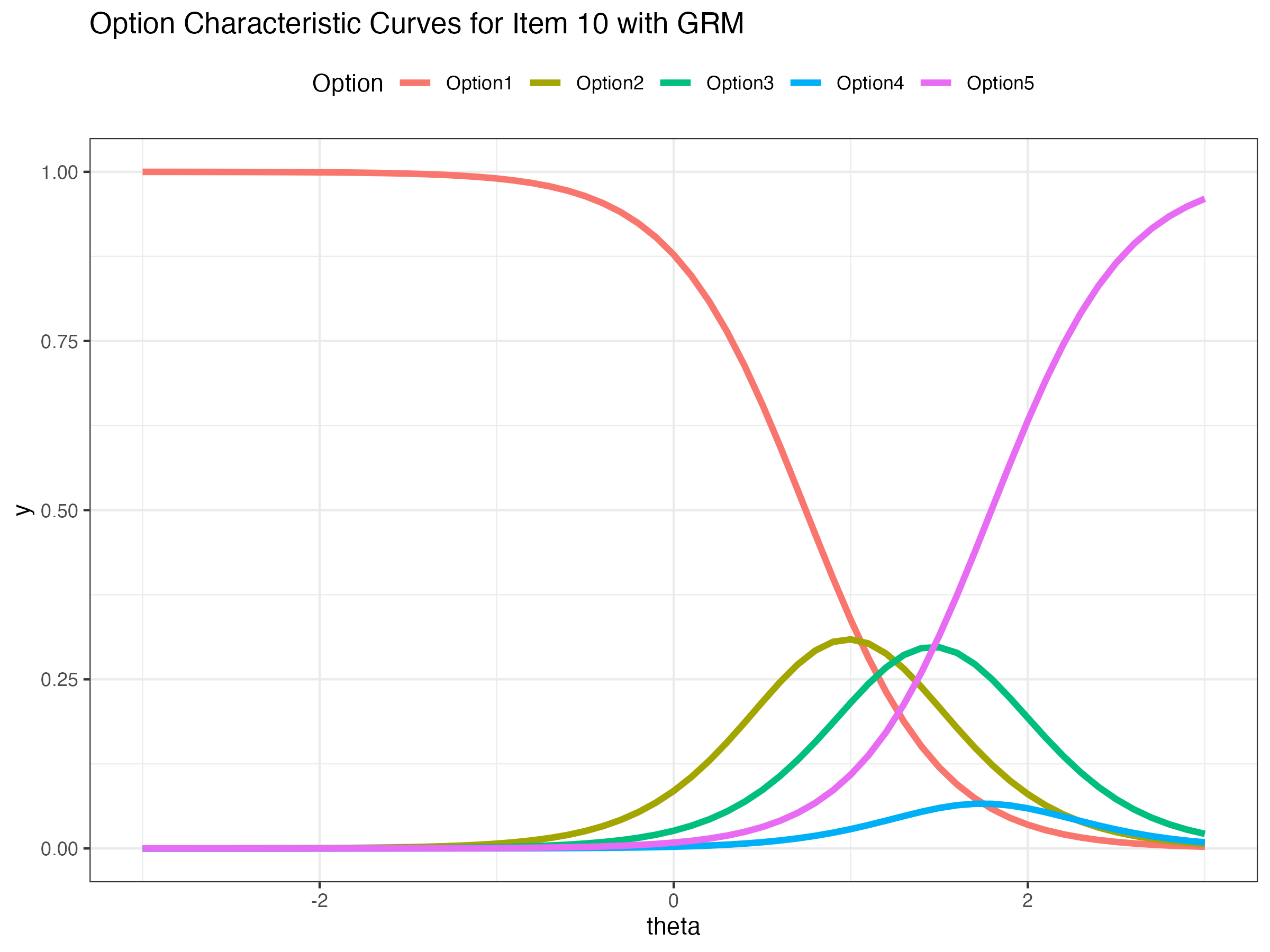{fig-align="center"}
## OPC for other 9 items
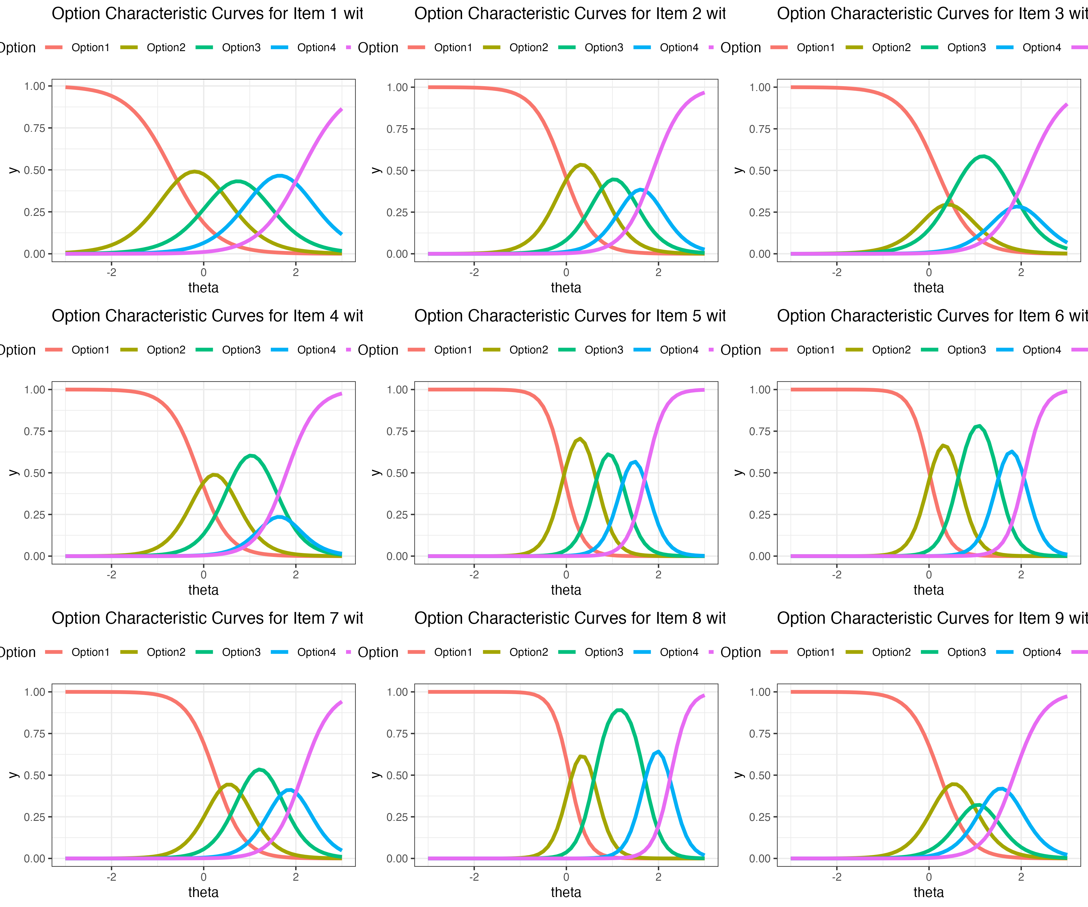{fig-align="center"}
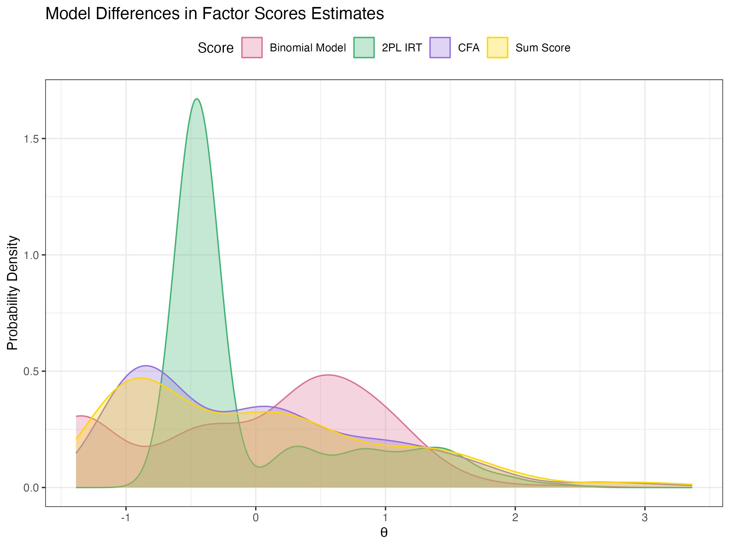
## EAP of Factor Scores for Four Models
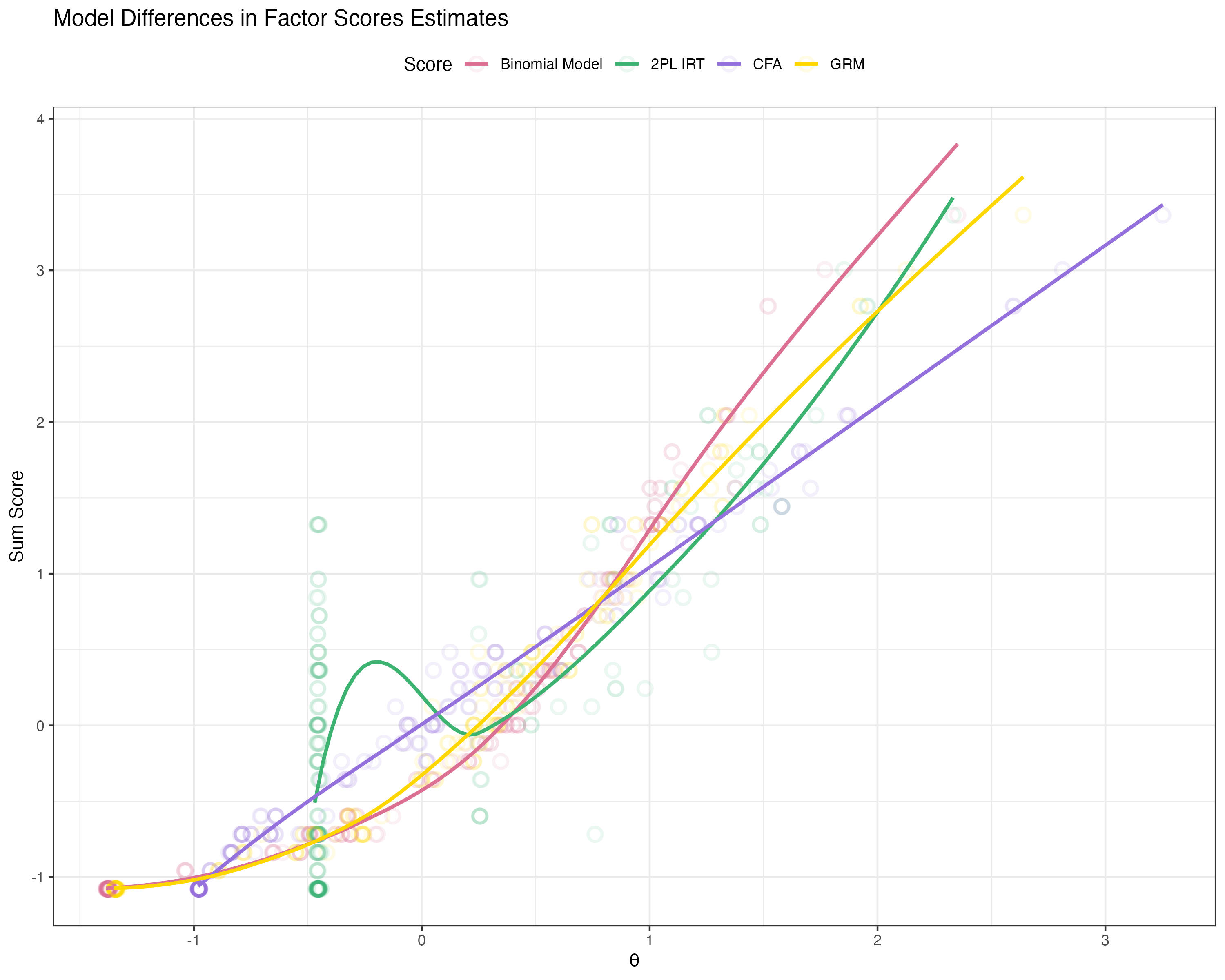{fig-align="center"}
## Posterior SDs around Factor Scores
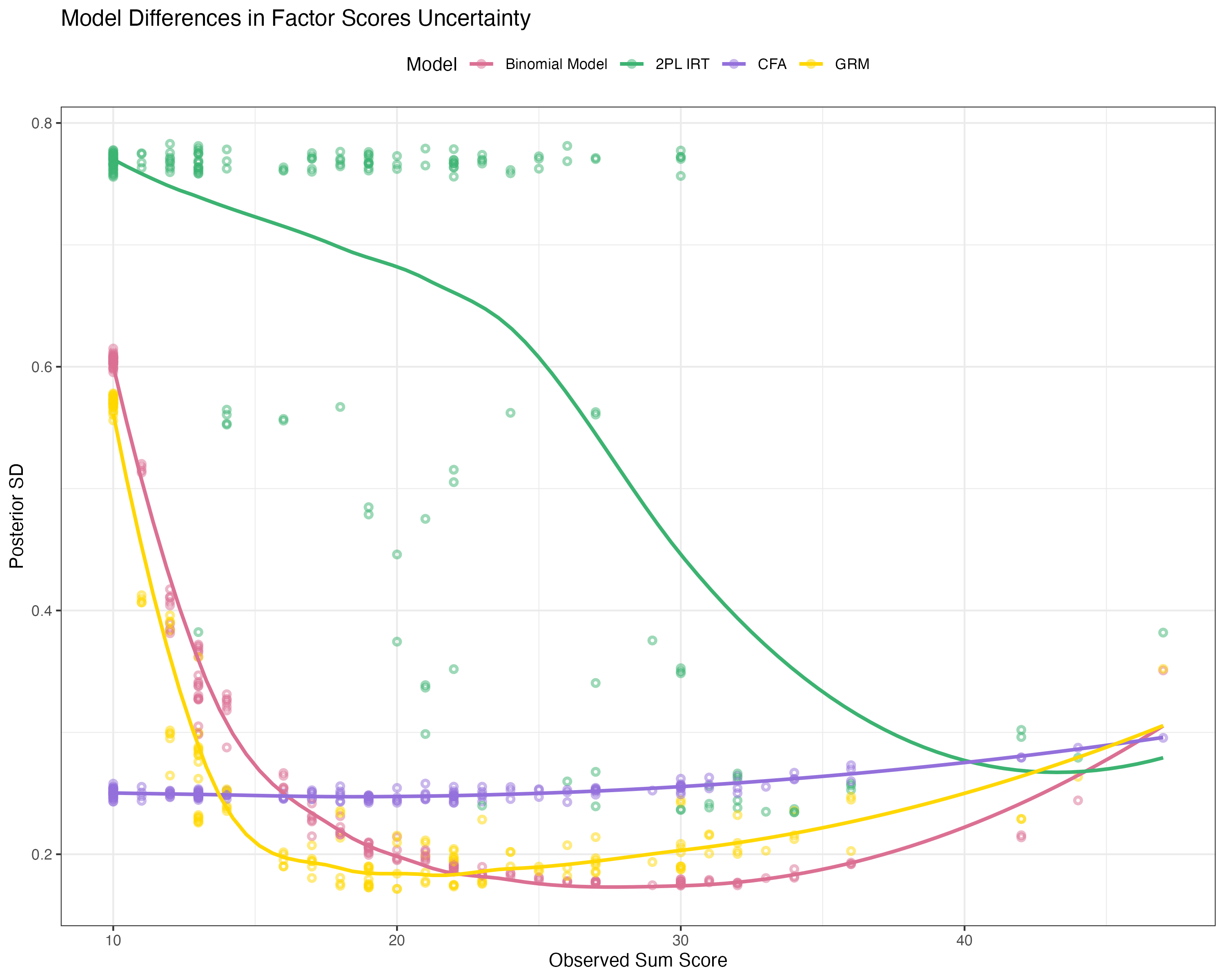{fig-align="center"}
## Resources
- [Dr. Templin's slide](https://jonathantemplin.github.io/Bayesian-Psychometric-Modeling-Course-Fall2022/lectures/lecture04d/04d_Modeling_Observed_Polytomous_Data#/binomial-model-data-block)