            Df Sum Sq Mean Sq F value Pr(>F)
group        1 218.42  218.42   264.1 <2e-16 ***
Residuals   38  31.43    0.83
---
Signif. codes: 0 '***' 0.001 '**' 0.01 '*' 0.05 '.' 0.1 ' ' 1Lecture 03: Introduction to One-way ANOVA
Experimental Design in Education
Jihong Zhang*, Ph.D
Educational Statistics and Research Methods (ESRM) Program*
University of Arkansas
2025-08-18
Lecture Outline
- Homework assignment
- Introduction to ANOVA
- Why use ANOVA instead of multiple t-tests?
- Logic and components of ANOVA
- Steps and assumptions in ANOVA
- Example scenario and real-world applications
- Performing ANOVA in R
- Checking homogeneity of variance
- Post-hoc analysis
- Using weights in ANOVA
- Where to find weights for ANOVA
- Conclusion
1 Homework 1
Let’s walk through HW1
2 One-Way ANOVA
Introduction
- Overview of ANOVA and its applications.
- Used for comparing means across multiple groups.
- Explanation of why ANOVA is essential in statistical analysis.
ANOVA Basics
Analysis of Variance (ANOVA) is a statistical method for comparing means across three or more groups.
When comparing only 2 groups, a t-test is typically used (though mathematically equivalent to ANOVA with 2 groups).
When comparing 3 or more groups, ANOVA using the F-test is the appropriate method to avoid inflating Type I error.
Why Use ANOVA Instead of Multiple t-tests?
- Computational efficiency: As the number of groups increases, the number of pairwise comparisons grows rapidly (k groups require k(k-1)/2 comparisons).
- Controls Type I error: Multiple t-tests inflate the family-wise error rate. For example, with 4 groups and α = 0.05, conducting 6 t-tests results in an actual error rate of approximately 0.26, not 0.05.
- Omnibus test: ANOVA provides a single test to determine if any group differences exist before conducting pairwise comparisons.
- Statistical power: ANOVA is more powerful than multiple t-tests when properly applied with post-hoc corrections.
Logic of ANOVA
ANOVA compares group means by analyzing variance components.
Two independent variance component estimates:
- Between-group variability: Differences among group means (reflects treatment effect)
- Within-group variability: Differences within each group (reflects random error or chance)
If the between-group variability is substantially larger than the within-group variability, we conclude that groups differ significantly.
Components of ANOVA
Total Sum of Squares (\(SS_{total}\)): Total variability in the outcome variable across all observations.
Sum of Squares Between (\(SS_{between}\)): Variability attributable to differences between group means (systematic variation).
Sum of Squares Within (\(SS_{within}\)): Variability within groups, representing random error (unsystematic variation).
- Key relationship: \(SS_{total} = SS_{between} + SS_{within}\)
If \(SS_{between}\) > \(SS_{within}\) …
Assume that we want to examine the effect of one drug on one disease (higher score means severity of the disease symptom). There are two group: one control group (placebo) and one treatment group.
The distributions of scores for two groups are like:
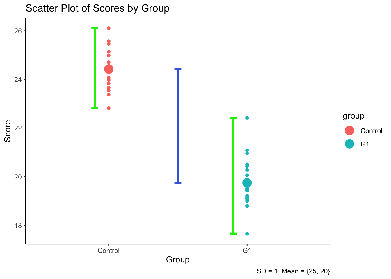
R output:
Interpretation: Residuals represents the within-group variability. group represents the between-group variability. With small within-group variability (SS = 31.43) and clear separation between groups, the F-statistic is large and highly significant. The between-group variance substantially exceeds the within-group variance, providing strong evidence that the groups differ.
If \(SS_{between}\) < \(SS_{within}\) …
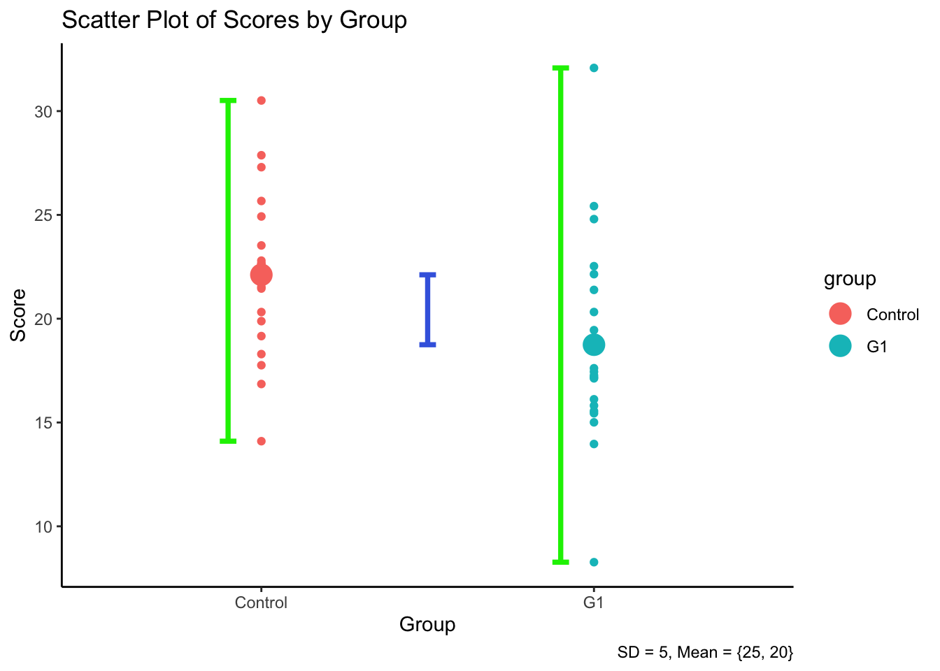
R output:
            Df Sum Sq Mean Sq F value Pr(>F)
group        1  113.4  113.43   5.485 0.0245 *
Residuals   38  785.8   20.68
---
Signif. codes: 0 '***' 0.001 '**' 0.01 '*' 0.05 '.' 0.1 ' ' 1Interpretation: With larger within-group variability (SS = 785.8), the overlap between groups increases. Even though the between-group variance remains the same, it is now smaller relative to the within-group variance. This results in a smaller F-statistic and reduced statistical power to detect group differences.
F-statistic check whether groups are separated on average, while for each group, samples are clustered within each group.
Practical Steps in One-way ANOVA
- Compute the total variability in the outcome variable.
- Partition the total variability into between-group (model) and within-group (error) components.
- Calculate the F-statistic: \(F_{obs} = \frac{SS_{between}/df_{between}}{SS_{within}/df_{within}}= \frac{MS_{between}}{MS_{within}}\)
- Construct the ANOVA table, set the alpha level (typically 0.05), and draw conclusions based on the p-value.
- Check the homogeneity of variance assumption (Levene’s test or Bartlett’s test).
- If the overall F-test is significant, conduct post-hoc pairwise comparisons (e.g., Tukey HSD) to identify which specific groups differ.
Assumptions of ANOVA
- Homogeneity of variance (homoscedasticity).
- Independence of observations.
- Normality of residuals.
Homogeneity of Variance
- Assumption: ANOVA assumes that the variance of the outcome variable is approximately equal across all groups (homoscedasticity).
- Why it matters: When variances differ substantially across groups, the F-test can become either too liberal (inflated Type I error) or too conservative (reduced power).
- Checking the assumption: Use visual inspection (boxplots), Levene’s test, or Bartlett’s test to assess variance equality before interpreting ANOVA results.
We will talk more details about this in the next lecture
Methods to Check Homogeneity of Variance
- Levene’s Test: Tests for equal variances across groups.
- Bartlett’s Test: Specifically tests for homogeneity in normally distributed data.
- Visual Inspection: Boxplots can help assess variance equality.
- Graph: Example of equal and unequal variance in boxplots.
When Homogeneity of Variance Is Violated
- Welch’s ANOVA (Welch’s F-test)
- Specifically designed for unequal variances
- Adjusts degrees of freedom to account for heteroscedasticity
- Generally preferred first option when HoV is violated
- Brown-Forsythe Test
- Another robust alternative to traditional ANOVA
- Less affected by unequal variances than standard F-test
- Non-parametric Alternatives
- Kruskal-Wallis test (non-parametric equivalent to one-way ANOVA)
- Does not assume equal variances or normality
- Tests for differences in distributions rather than means
3 Example: One-way ANOVA in R
Example Scenario
- Research Aim: Investigating the effect of a teaching intervention on children’s verbal acquisition.
- IV (Factor): Intervention groups (G1, G2, G3, Control).
- DV: Verbal acquisition scores.
- Hypotheses:
- \(H_0\): \(\mu_{Control} = \mu_{G1} = \mu_{G2} = \mu_{G3}\)
- \(H_A\): At least two group means differ.
Performing ANOVA in R
Load R packages
Generate Sample Data
 [1]  7.929343 22.774292 30.844412 -3.456977 24.291247 25.060559 14.252600
[8] 14.533681 14.355480 11.099622Explanation: The rnorm() function generates random values from a normal distribution. The set.seed() function ensures reproducibility by fixing the random number generation sequence.
Context: This example focuses on whether three different teaching methods (labeled as G1, G2, G3) affect students’ test scores.
In total, 40 students are assigned to three teaching groups and one control group. Each group has 10 students.
set.seed(1234)
# Create dataset with EQUAL variances (SD = 5 for all groups)
data <- data.frame(
  group = rep(c("G1", "G2", "G3", "Control"), each = 10),
  score = c(rnorm(10, 20, 5), rnorm(10, 25, 5), rnorm(10, 30, 5), rnorm(10, 22, 5))
)
# Create dataset with UNEQUAL variances (SD varies from 0.1 to 10 across groups)
data_unequal <- data.frame(
  group = rep(c("G1", "G2", "G3", "Control"), each = 10),
  score = c(rnorm(10, 20, 10), rnorm(10, 25, 5), rnorm(10, 30, 1), rnorm(10, 22, .1))
)Note: We create two datasets to demonstrate the importance of homogeneity of variance:
data: Equal variances (homoscedastic) - meets ANOVA assumptionsdata_unequal: Unequal variances (heteroscedastic) - violates ANOVA assumptions
Conduct ANOVA Test
            Df Sum Sq Mean Sq F value   Pr(>F)
group        3  724.1  241.37   11.45 2.04e-05 ***
Residuals   36  759.2   21.09
---
Signif. codes: 0 '***' 0.001 '**' 0.01 '*' 0.05 '.' 0.1 ' ' 1 Df Sum Sq Mean Sq F value Pr(>F)
group 3 1413 470.9 19.14 1.37e-07 ***
Residuals 36 886 24.6
---
Signif. codes: 0 '***' 0.001 '**' 0.01 '*' 0.05 '.' 0.1 ' ' 1Comparison: - Both ANOVAs show significant F-statistics (p < 0.05), indicating group differences - However, the unequal variance dataset violates ANOVA assumptions, making these results potentially unreliable - For data_unequal, we should use Welch’s ANOVA instead: oneway.test(score ~ group, data = data_unequal)
In-class Exercise: compare between and within SS
Interactive Exercise
This exercise uses WebR to run R code directly in your browser. Click “Run Code” to execute the code and see the results. You can also modify the code and re-run it to explore different scenarios!
Research Context
A psychology researcher is investigating the effectiveness of different study techniques on exam performance. The researcher randomly assigns 60 college students to three different study groups:
- Group 1 (Spaced Practice): Students study material across multiple sessions over several weeks
- Group 2 (Massed Practice): Students study material in intensive “cramming” sessions
- Group 3 (Mixed Practice): Students use a combination of spaced and massed practice
Each group contains 20 students. The researcher measures final exam scores (0-100 scale).
Exercise Questions
- Simulate data for two scenarios:
- Scenario A: Study technique has a strong effect (large between-group variance relative to within-group variance)
- Scenario B: Study technique has a weak effect (small between-group variance relative to within-group variance)
- For each scenario:
- Calculate \(SS_{between}\) and \(SS_{within}\)
- Compute the F-statistic
- Interpret whether study technique significantly affects exam performance
Scenario A: Strong Treatment Effect
Your Task: Complete the code below by filling in the missing sections to conduct ANOVA and extract variance components.
Hints for completing the exercise
- Conduct ANOVA: Use
aov([Outcome_Name] ~ [Group_Name], data = data_strong)to run the analysis - Get summary: Use
summary()on the ANOVA result
Complete Solution with Full Code:
Interpretation (Click to expand)
Variance Components:
When you run the code above, you’ll observe:
- \(MS_{between}\) is substantially larger (variability due to different study techniques)
- \(MS_{within}\) is relatively small (variability within each group)
Statistical Results:
The F-statistic will be large and highly significant (p < .001).
Conclusion:
The between-group variability is much larger than the within-group variability. This indicates that study technique has a strong and significant effect on exam performance. The F-statistic is very large and highly significant, providing strong evidence that at least two study techniques produce different mean exam scores.
The groups are well-separated, with minimal overlap. Students within each group perform similarly to each other (small \(SS_{within}\)), but there are substantial differences between the average performance of different study technique groups (large \(SS_{between}\)).
Scenario B: Weak Treatment Effect
Your Task: Complete the code below by filling in the missing sections to conduct ANOVA and extract variance components.
Hints for completing the exercise
- Conduct ANOVA: Use
aov(score ~ group, data = data_weak)to run the analysis - Get summary: Use
summary()on the ANOVA result
Question to consider: How do the variance components in this scenario compare to Scenario A? What does this tell you about the treatment effect?
Complete Solution with Full Code:
Interpretation (Click to expand)
Variance Components:
When you run the code above, you’ll observe:
\(SS_{between}\) and \(MS_{between}\) and relatively small (variability due to different study techniques)
\(SS_{within}\) and \(MS_{within}\) are substantially larger (variability within each group)
Statistical Results:
The F-statistic will be small and not statistically significant (p > .05).
Conclusion:
The between-group variability is much smaller than the within-group variability. This indicates that study technique has little to no effect on exam performance. The F-statistic is small and not statistically significant, providing insufficient evidence to conclude that study techniques differ in their effectiveness.
There is substantial overlap between groups. The variability in exam scores within each study technique group is large (\(SS_{within}\)), overwhelming any small differences that might exist between the average performance of different groups (\(SS_{between}\)). Individual differences among students (captured by \(SS_{within}\)) are more important than the study technique they used.
Key Takeaways from Exercise
Understanding the Ratio \(MS_{between} / MS_{within}\)
Large ratio (Scenario A): When \(MS_{between} \gg MS_{within}\), the treatment effect is strong and detectable. Groups are well-separated with minimal within-group variability.
Small ratio (Scenario B): When \(MS_{between} \ll MS_{within}\), the treatment effect is weak and difficult to detect. Groups overlap substantially due to large within-group variability.
The F-statistic is essentially this ratio (adjusted for degrees of freedom): \[F = \frac{MS_{between}}{MS_{within}} = \frac{SS_{between}/df_{between}}{SS_{within}/df_{within}}\]
Practical implication: To detect treatment effects, researchers should:
- Maximize between-group differences (strong manipulation)
- Minimize within-group variance (careful measurement, homogeneous samples, experimental control)
Checking Homogeneity of Variance (HoV)
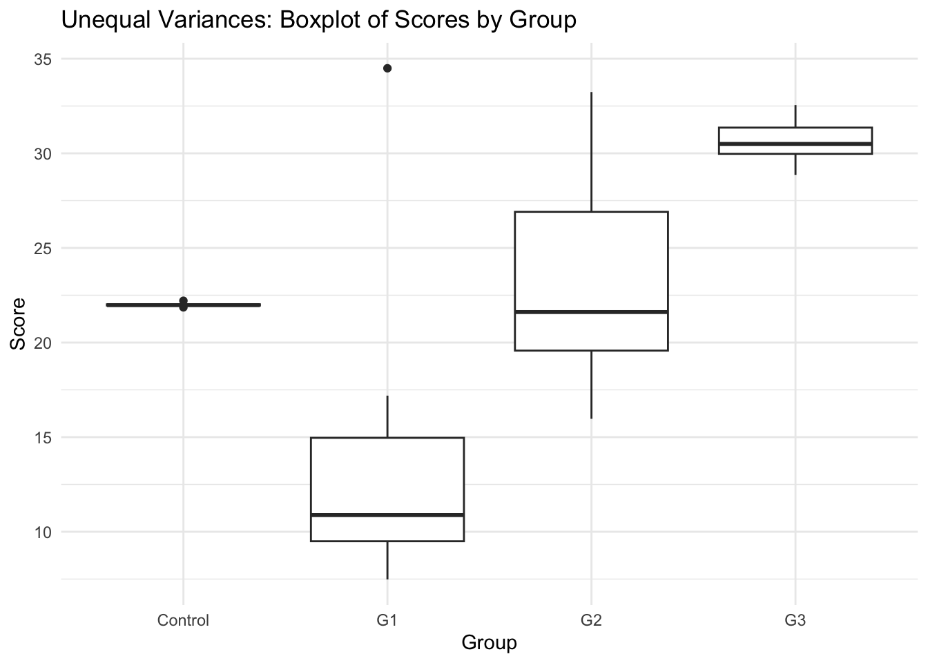
Method 1: Visual Inspection
Equal Variances across groups
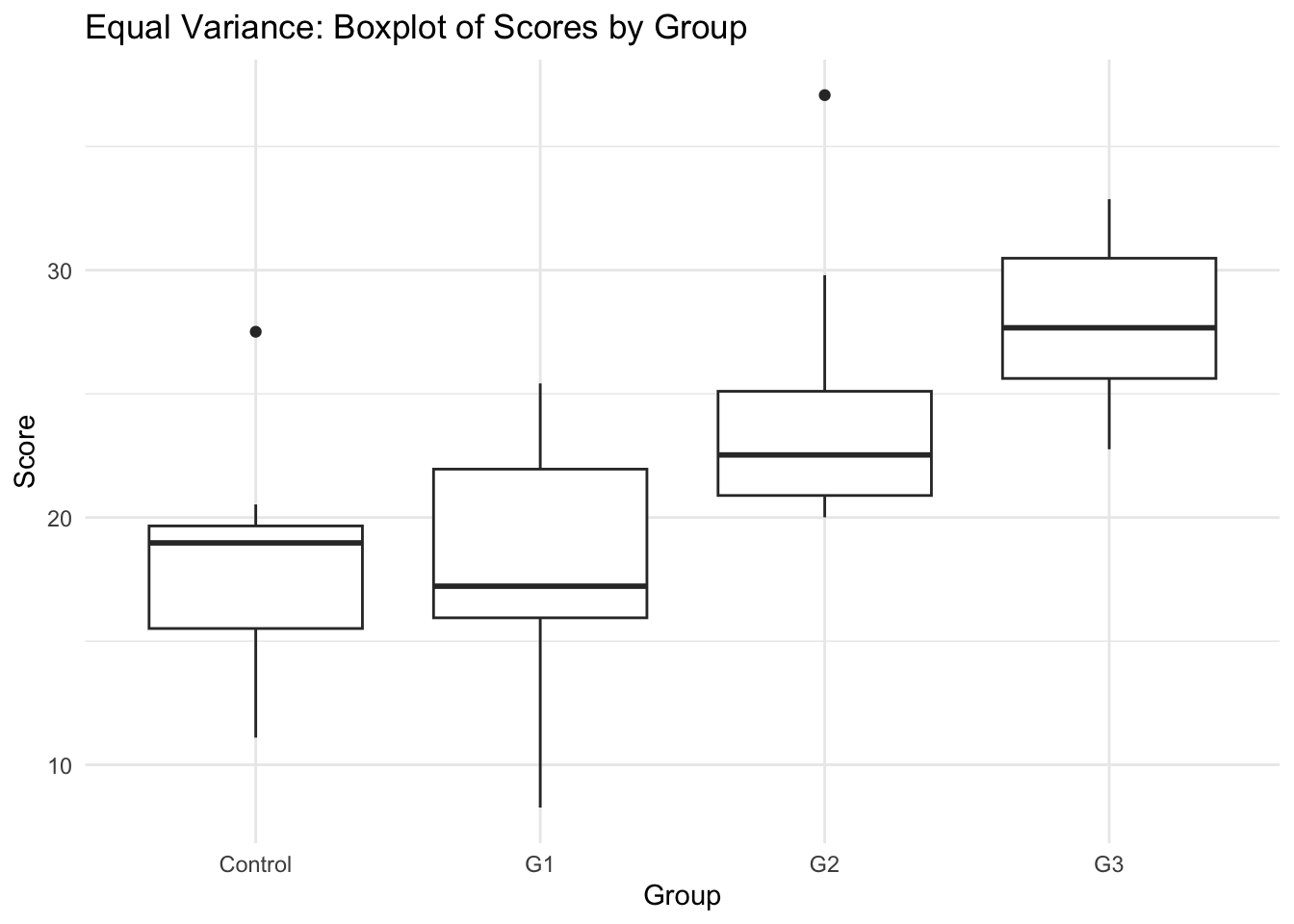
Unequal Variances across groups
Method 2: Using Bartlett’s Test
Null Hypothesis (\(H_0\)): Groups are same within-group variability.
Equal group:

    Bartlett test of homogeneity of variances

data:  score by group
Bartlett's K-squared = 2.0115, df = 3, p-value = 0.57

Unequal group:

    Bartlett test of homogeneity of variances

data:  score by group
Bartlett's K-squared = 82.755, df = 3, p-value < 2.2e-16Interpretation:
- Equal variance data: The Bartlett test is non-significant (p > 0.05), indicating we have no evidence against the null hypothesis. We can assume the groups have homogeneous variances.
- Unequal variance data: The Bartlett test is significant (p < 0.05), indicating strong evidence that variances differ across groups. This violates the homogeneity of variance assumption, and we should consider using Welch’s ANOVA or other robust alternatives.
Method 3: Using Levene’s Test
Levene's Test for Homogeneity of Variance (center = median)
      Df F value Pr(>F)
group  3  0.1779 0.9107
36 Levene's Test for Homogeneity of Variance (center = median)
Df F value Pr(>F)
group 3 3.4749 0.02581 *
36
---
Signif. codes: 0 '***' 0.001 '**' 0.01 '*' 0.05 '.' 0.1 ' ' 1Interpretation:
- Equal variance data: Levene’s test shows p > 0.05, confirming homogeneity of variance across groups.
- Unequal variance data: Levene’s test shows p < 0.05, indicating significant differences in variances. This suggests the homogeneity assumption is violated and alternative methods should be considered.
When to use each test
Use Levene’s Test (more frequently used) when:
- Data may not be normally distributed
- Dealing with outliers in the dataset
- Working with small sample sizes
- Conducting preliminary tests for ANOVA with non-normal data
- General robustness is prioritized over power
Use Bartlett’s Test when:
- Data is confirmed to be normally distributed
- No significant outliers are present
- Larger sample sizes are available
- Maximum statistical power is desired (under normality)
- Preliminary testing for parametric procedures with normal data
Real-world Applications of ANOVA
- Experimental designs in psychology.
- Clinical trials in medicine.
- Market research and A/B testing.
- Example case studies.
Using Weights in ANOVA
- In some cases, observations may have different levels of reliability or importance.
- Weighted ANOVA allows us to account for these differences by assigning weights.
- Example: A study where some groups have higher variance and should contribute less to the analysis.
Correct Approach to Sampling Weights
Basic Principle
- Inverse weighting: Weight = 1 / (Selection probability)
- Clusters with larger samples have higher selection probabilities
- Therefore, they receive smaller weights
Example
- If Cluster A has 1000 people and you sampled 100, selection probability = 100/1000 = 0.1
- If Cluster B has 100 people and you sampled 50, selection probability = 50/100 = 0.5
- Weight for Cluster A = 1/0.1 = 10
- Weight for Cluster B = 1/0.5 = 2
Why This Works
- Oversampled groups (higher sampling fraction) get downweighted
- Undersampled groups (lower sampling fraction) get upweighted
- This corrects the disproportionate representation in your sample
Example: Applying Weights in aov()
            Df Sum Sq Mean Sq F value   Pr(>F)
group        3  666.6  222.20   7.578 0.000471 ***
Residuals   36 1055.5   29.32
---
Signif. codes: 0 '***' 0.001 '**' 0.01 '*' 0.05 '.' 0.1 ' ' 1Interpretation:
- The weights modify the influence of each observation in the model. In this example, G2 observations receive double weight (2.0), G3 observations receive half weight (0.5), and G1 and Control receive standard weights.
- Notice how the F-statistic and p-value change compared to the unweighted analysis, reflecting the differential contribution of each group.
- This approach is useful when data reliability varies across groups or when correcting for sampling design effects.
Where Do We Get Weights for ANOVA?
- Weights can be derived from:
- Large-scale assessments: Different student groups may have varying reliability in measurement.
- Survey data: Unequal probability of selection can be adjusted using weights.
- Experimental data: Measurement error models may dictate different weight assignments.
Example: Using Weights in Large-Scale Assessments
- Consider an educational study where test scores are collected from schools of varying sizes.
- Larger schools may contribute more observations but should not dominate the analysis.
- Weighting adjusts for this imbalance:
            Df Sum Sq Mean Sq F value   Pr(>F)
group        3  724.1  241.37   11.45 2.04e-05 ***
Residuals   36  759.2   21.09
---
Signif. codes: 0 '***' 0.001 '**' 0.01 '*' 0.05 '.' 0.1 ' ' 1Interpretation:
- In this example, we apply conditional weighting where observations from “LargeSchool” receive half the weight (0.5) compared to other groups (weight = 1).
- This prevents larger schools from dominating the analysis due to their overrepresentation in the sample.
- The weighted analysis ensures fair representation across schools of different sizes, providing more generalizable results.
Conclusion and Interpretation
- Review results and discuss findings.
- Key takeaways from the analysis.

ESRM 64503