Lecture 02: Hypothesis Testing

Experimental Design in Education

Jihong Zhang*, Ph.D

Educational Statistics and Research Methods (ESRM) Program*

University of Arkansas

2025-08-18

Presentation Outline

• Types of Statistics
  • Descriptive: Summarize data (central tendency, variability, shape)
  • Inferential: Make population inferences from samples
  • Predictive: Make predictions for new data
• Hypothesis Testing Steps
  1. State \(H_0\) and \(H_A\)
  2. Set \(\alpha\) level
  3. Compute test statistics
  4. Conduct test and make decision
• ANOVA Fundamentals
  • One dependent variable (DV), one independent variable (IV) with multiple levels
  • Between-subjects and within-subjects designs
  • Interaction effects
• Test Components
  • Error types (Type I and Type II)
  • Variance decomposition (\(SS_{Total}\), \(SS_{Between}\), \(SS_{Within}\))
  • F-statistics and critical values
• Examples
  • Political attitudes study
  • Sleep and academic performance study
• Decision Making
  • Compare \(F_{observed}\) vs \(F_{critical}\)
  • Compare p-value vs \(\alpha\)
  • Interpret at \((1-\alpha)\) confidence level

Types of Statistics

Statistics can be classified by purpose:

1. Descriptive Statistics
2. Inferential Statistics
3. Predictive Statistics

1. Descriptive Statistics

• Definition: Describes and summarizes the collected data using numbers/values
  • Central tendency: mean, median, mode
  • Variability: range, interquartile range (IQR), variance, standard deviation
  • Shape of distribution: skewness, kurtosis

# install.packages("moments")
moments::skewness(c(1:10, 100))

[1] 2.793716

moments::skewness(rnorm(100, 0, 1)) # should be close to 0

[1] -0.1416608

• Examples of skewness with two graphs:

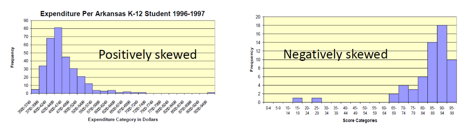
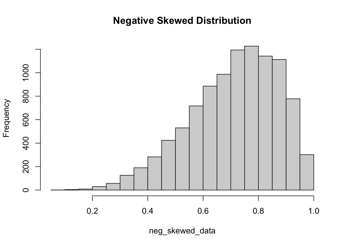
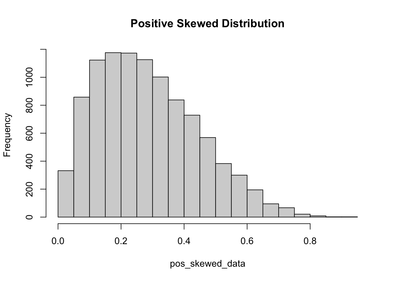
Examples of positive and negative skewness in distributions

set.seed(1234)
# Simulate a skewed normal distribution using beta distribution
neg_skewed_data <- rbeta(10000,5,2)
hist(neg_skewed_data, main = "Negative Skewed Distribution")

pos_skewed_data <- rbeta(10000,2,5)
hist(pos_skewed_data, main = "Positive Skewed Distribution")

library(ggplot2)
library(tidyr)
data.frame(
  neg = neg_skewed_data,
  pos = pos_skewed_data
  ) |>
  pivot_longer(c(neg, pos), names_to = "Type") |> 
  ggplot(aes(y = value, fill = Type)) +
  geom_boxplot() +
  scale_fill_discrete(labels = c("Negative Skewed", "Positive Skewed"), name = "")

2. Inferential Statistics

• Definition: Uses probability theory to infer/estimate population characteristics from a sample using hypothesis testing
• Visual representation shows:
  • Population → Sampling → Sample
  • Sample → Inference → Population
    • Sample is analyzed using descriptive statistics
    • Inferential statistics used to make conclusions about population

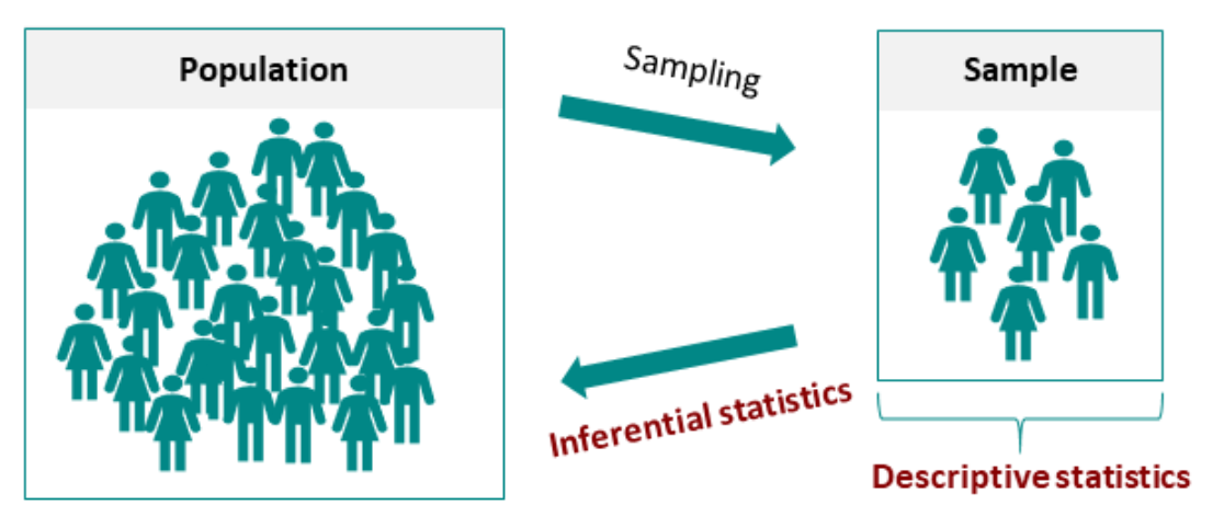
The relationship between population, sample, and inference

3. Predictive Statistics

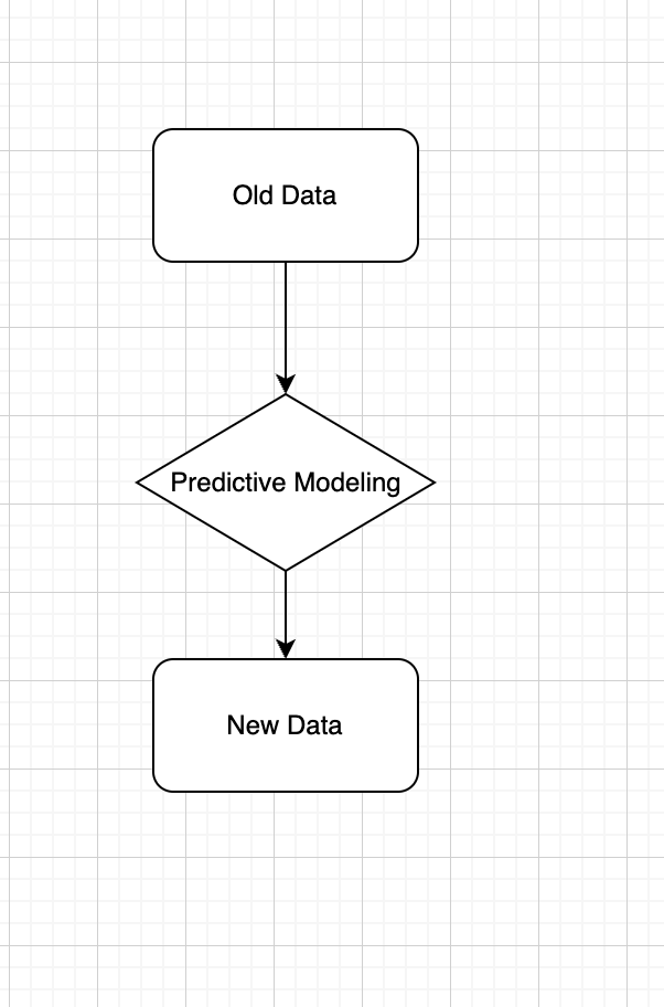
• Definition: Use observed data to produce the most accurate prediction possible for new data. Here, the primary goal is that the predicted values have the highest possible fidelity to the true value of the new data.

• Example: A simple example would be for a book buyer to predict how many copies of a particular book should be shipped to their store for the next month.

Example of predictive statistics workflow

Which type of statistics to use

1. How many houses burned in California wildfire in the first week?

   • Descriptive

2. Which factor is most important causing the fires?

   • Inference

3. How likely the California wildfire will not happen again in next 5 years?

   • Predictive

4. How likely human will live on Mars?

   • Not statistics. Sci-Fi

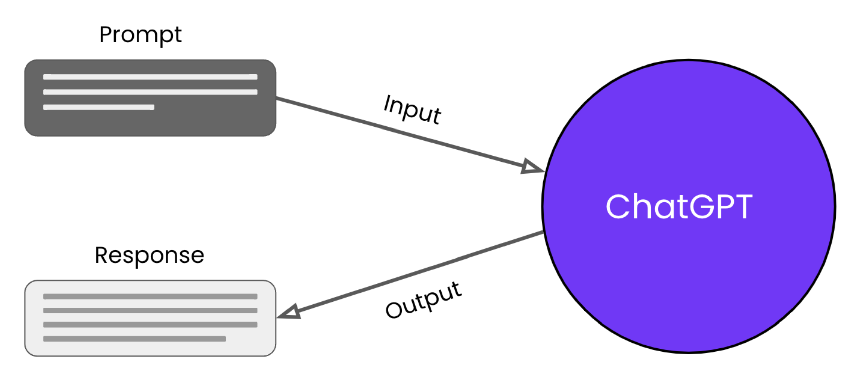
5. Which type of statistics is used by ChatGPT?

   ChatGPT uses predictive statistics for text generation

Statistical Hypothesis Testing Steps

Steps for Inferential Statistical Testing:

1. State null hypothesis (\(H_0\)) and alternative hypothesis (\(H_A\))
   • Null hypothesis must be some statement that is statistically testable.
2. Set alpha α (type I error rate) to determine significance levels
   • rejection region vs. p-value
3. Compute test statistics (i.e., F-statistics)
4. Conduct hypothesis testing:
   • Compare test statistics: critical value vs. observed value
   • Compare alpha and p-value

ANOVA Introduction

• ANOVA is one of the most frequently used statistical tool for inferential statistics in experimental design.
• Settings for Analysis of Variance (ANOVA):
  • One dependent variable (DV), “Outcome”
  • One independent variable (IV) with multiple levels, “Group”
• Example question: “Are there mean differences in SAT math scores (outcome) for different high school program types (group)?”
• Course covers advanced ANOVA topics:
  • Group comparisons (Group A vs. B vs. C)
  • Model comparisons
  • Between/within-subject design
  • Interaction effects

Types of ANOVA: Key Differences

• One-Way ANOVA

  • Purpose: Tests one factor with three or more levels on a continuous outcome.

  • Use Case: Comparing means across multiple groups (e.g., diet types on weight loss).

• Two-Way ANOVA

  • Purpose: Examines two factors and their interaction on a continuous outcome.

  • Use Case: Studying effects of diet and exercise on weight loss.

• Repeated Measures ANOVA

  • Purpose: Tests the same subjects under different conditions or time points.

  • Use Case: Longitudinal studies measuring the same outcome over time (e.g., cognitive tests after varying sleep durations).

• Mixed-Design ANOVA

  • Purpose: Combines between-subjects and within-subjects factors in one analysis.

  • Use Case: Evaluating treatment effects over time with control and experimental groups.

• Multivariate Analysis of Variance (MANOVA)

  • Purpose: Assesses multiple continuous outcomes (dependent variables) influenced by independent variables.

  • Use Case: Impact of psychological interventions on anxiety, stress, and self-esteem.

1 Example 1: Political Study on Tax Reform Attitudes

Background

• A political scientist studies tax reform attitudes across political groups:
  • Groups: Democrats (n=4), Republicans (n=5), Independents (n=8)
  • Outcome measure: Attitude scores (higher score = greater concern for tax reform)
  • Analysis: Conducted at \(\alpha = .05\)
  • Variables:
    • party: Political affiliation
    • scores: Attitude scores for survey respondents

## Install the package ESRM64103 from GitHub
remotes::install_github("JihongZ/ESRM64103")

library(ESRM64103)
library(dplyr)
exp_political_attitude

         party scores
1     Democrat      4
2     Democrat      3
3     Democrat      5
4     Democrat      4
5     Democrat      4
6   Republican      6
7   Republican      5
8   Republican      3
9   Republican      7
10  Republican      4
11  Republican      5
12 Independent      8
13 Independent      9
14 Independent      8
15 Independent      7
16 Independent      8

Workflow of data analysis in R

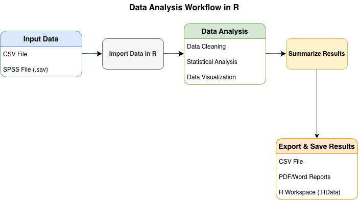
Data Analysis Workflow in R

Descriptive Statistics: Summary Statistics

• Calculate mean, standard deviation, and variance for each political group

• Grand mean across all groups: 5.625

# Grand mean
mean(exp_political_attitude$scores)

[1] 5.625

exp_political_attitude$party <- factor(exp_political_attitude$party, 
                                       levels = c("Democrat", "Republican", "Independent"))
mean_byGroup <- exp_political_attitude |> 
  group_by(party) |> 
  summarise(Mean = mean(scores),
            SD = round(sd(scores), 2),
            Vars = round(var(scores), 2),
            N = n())
mean_byGroup

# A tibble: 3 × 5
  party        Mean    SD  Vars     N
  <fct>       <dbl> <dbl> <dbl> <int>
1 Democrat        4  0.71   0.5     5
2 Republican      5  1.41   2       6
3 Independent     8  0.71   0.5     5

Descriptive Statistics: Bar Plot

library(ggplot2)
ggplot(data = mean_byGroup) +
  geom_bar(mapping = aes(x = party, y = Mean, fill = party), stat = "identity", width = .5) +
  geom_label(aes(x = party, y = Mean, label = Mean), nudge_y = .3) +
  labs(title = "Attitudes Toward the Tax Return") +
  theme(text = element_text(size = 15))

Descriptive Statistics: Multiple Variables

In research, we often need to compute descriptive statistics for multiple continuous variables simultaneously. Here are several approaches:

# Generate simulated student performance data
set.seed(2025)
n_students <- 100

student_data <- data.frame(
  student_id = 1:n_students,
  math_score = rnorm(n_students, mean = 75, sd = 12),
  reading_score = rnorm(n_students, mean = 78, sd = 10),
  science_score = rnorm(n_students, mean = 72, sd = 11),
  study_hours = rgamma(n_students, shape = 2, scale = 3),
  attendance_rate = rbeta(n_students, shape1 = 8, shape2 = 2) * 100
)

Method 1: Base R with sapply()

# Select only continuous variables
continuous_vars <- student_data[, c("math_score", "reading_score", "science_score", "study_hours", "attendance_rate")]

# Compute mean, sd, and range for each variable
desc_stats <- data.frame(
  Mean = sapply(continuous_vars, mean),
  SD = sapply(continuous_vars, sd),
  Min = sapply(continuous_vars, min),
  Max = sapply(continuous_vars, max),
  Range = sapply(continuous_vars, function(x) max(x) - min(x))
)

round(desc_stats, 2)

                 Mean    SD   Min    Max Range
math_score      74.94 12.24 45.59 109.23 63.64
reading_score   78.09  9.65 58.84 100.50 41.66
science_score   72.10 10.83 40.66  99.39 58.73
study_hours      6.03  4.81  0.40  26.14 25.74
attendance_rate 80.53 10.53 49.08  99.10 50.02

Method 2: Using dplyr package with across()

library(dplyr)

student_data |>
  summarise(
    across(
      c(math_score, reading_score, science_score, study_hours, attendance_rate),
      list(
        Mean = ~mean(.x),
        SD = ~sd(.x),
        Min = ~min(.x),
        Max = ~max(.x),
        Range = ~max(.x) - min(.x)
      ),
      .names = "{.col}_{.fn}"
    )
  ) |>
  tidyr::pivot_longer(
    everything(),
    names_to = c("Variable", "Statistic"),
    names_sep = "_(?=[^_]+$)",
    values_to = "Value"
  ) |>
  tidyr::pivot_wider(
    names_from = Statistic,
    values_from = Value
  ) |>
  mutate(across(where(is.numeric), ~round(.x, 2)))

# A tibble: 5 × 6
  Variable         Mean    SD   Min   Max Range
  <chr>           <dbl> <dbl> <dbl> <dbl> <dbl>
1 math_score      74.9  12.2   45.6 109.   63.6
2 reading_score   78.1   9.65  58.8 100.   41.7
3 science_score   72.1  10.8   40.7  99.4  58.7
4 study_hours      6.03  4.81   0.4  26.1  25.7
5 attendance_rate 80.5  10.5   49.1  99.1  50.0

Method 3: Using psych::describe()

The psych package provides a comprehensive describe() function:

library(psych)

continuous_vars |>
  describe() |>
  select(n, mean, sd, min, max, range) |>
  round(2)

                  n  mean    sd   min    max range
math_score      100 74.94 12.24 45.59 109.23 63.64
reading_score   100 78.09  9.65 58.84 100.50 41.66
science_score   100 72.10 10.83 40.66  99.39 58.73
study_hours     100  6.03  4.81  0.40  26.14 25.74
attendance_rate 100 80.53 10.53 49.08  99.10 50.02

Grouped Descriptive Statistics

You can also compute descriptives by groups:

# Add a grouping variable
student_data$program <- sample(c("STEM", "Arts", "Social Sciences"),
                               n_students, replace = TRUE,
                               prob = c(0.4, 0.3, 0.3))

# Compute descriptives by program
student_data |>
  group_by(program) |>
  summarise(
    N = n(),
    Math_Mean = mean(math_score),
    Math_SD = sd(math_score),
    Reading_Mean = mean(reading_score),
    Reading_SD = sd(reading_score),
    Science_Mean = mean(science_score),
    Science_SD = sd(science_score)
  ) |>
  mutate(across(where(is.numeric) & !N, ~round(.x, 2)))

# A tibble: 3 × 8
  program             N Math_Mean Math_SD Reading_Mean Reading_SD Science_Mean
  <chr>           <int>     <dbl>   <dbl>        <dbl>      <dbl>        <dbl>
1 Arts               30      74.2    12.7         80.5       10.1         72.8
2 STEM               44      74.3    12.4         77.6        9.1         73.4
3 Social Sciences    26      76.9    11.7         76.1        9.8         69.2
# ℹ 1 more variable: Science_SD <dbl>

Workflow of Example 1

remotes::install_github("JihongZ/ESRM64103")
library(ESRM64103)
library(dplyr)
exp_political_attitude
exp_political_attitude$party <- factor(exp_political_attitude$party, 
                                       levels = c("Democrat", "Republican", "Independent"))
mean_byGroup <- exp_political_attitude |> 
  group_by(party) |> 
  summarise(Mean = mean(scores),
            SD = round(sd(scores), 2),
            Vars = round(var(scores), 2),
            N = n())
mean_byGroup
anova_model <- lm(scores ~ party, data = exp_political_attitude)
anova(anova_model)

Steps of ANOVA

1. State the null hypothesis and alternative hypothesis:

   • \(H_0\): \(\bar{X}_{dem}\) = \(\bar{X}_{rep}\) = \(\bar{X}_{ind}\)
   • \(H_A\): At least two groups are significantly different
   • Question: Why not testing \(\bar{SD}_{dem}\) = \(\bar{SD}_{rep}\) = \(\bar{SD}_{ind}\)?
   • Answer: You definitely can in statistics. Variances homogeneity.

2. Set the significant alpha = 0.05

3. Calculate Observed F-statistics:

   \[ F_{obs} = \frac{SS_b/df_b}{SS_w/df_w} \]

   • Degrees of freedom: \(df_b\) = 3 (groups) - 1 = 2, \(df_w\) = 16 (samples) - 3 (groups) = 13

   • Between-group sum of squares: \[SS_b = \sum_{j=1}^{g} n_j(\bar{Y}_j - \bar{Y})^2 = 43.75\] where \(n_j\) is group sample size, \(\bar{Y}_j\) is group mean, and \(\bar{Y}\) is the grand mean.

   • Within-group sum of squares: \[SS_w = \sum_{j=1}^{3} \sum_{i=1}^{n_j}(Y_{ij}-\bar{Y}_j)^2 = 14.00\] where \(Y_{ij}\) is individual \(i\)’s score in group \(j\).

R code to calcuate F statistics

GrandMean <- mean(exp_political_attitude$scores)
## Between-group Sum of Squares
cat("Between-group Sum of Squares: ", sum(mean_byGroup$N * (mean_byGroup$Mean - GrandMean)^2))

Between-group Sum of Squares:  43.75

## Within-group Sum of Squares
SSw_dt <- exp_political_attitude |> 
  group_by(party) |> 
  mutate(GroupMean = mean(scores),
         Diff_sq = (scores - GroupMean)^2) 

cat("Within-group Sum of Squares: ", sum(SSw_dt$Diff_sq))

Within-group Sum of Squares:  14

SS_b <- sum(mean_byGroup$N * (mean_byGroup$Mean - GrandMean)^2)
SS_w <- sum(SSw_dt$Diff_sq)
df_b = 2
df_w = 16 - 3 
F_bw = (SS_b / df_b) / (SS_w / df_w)

• \(F_{critical}\) (df_num = 2, df_deno = 13) = 3.81
• \(F_{observed}\) = 20.31

anova_model <- lm(scores ~ party, data = exp_political_attitude)
anova(anova_model)

Analysis of Variance Table

Response: scores
          Df Sum Sq Mean Sq F value    Pr(>F)    
party      2  43.75 21.8750  20.312 9.994e-05 ***
Residuals 13  14.00  1.0769                      
---
Signif. codes:  0 '***' 0.001 '**' 0.01 '*' 0.05 '.' 0.1 ' ' 1

Results show rejection of \(H_0\) (\(F_{obs}\) > \(F_{critical}\))

Step 1: State the null hypothesis and alternative hypothesis

1. Formulate the null hypothesis (\(H_0\)) and the alternative hypothesis (\(H_A\))
   • Prior to any statistical tests, start with a working hypothesis based on an initial guess about the phenomenon.
   • Example: Investigating whether political groups affect their attitudes.
     • Research question: “Is there a variance in attitude score among different groups?”
     • Hypothesis: “Different political groups will show varied attitudes.”
   • Operational Definitions:
     • Null hypothesis (\(H_0\)): No observed difference or effect (“Something is something”).
       • Group A’s mean - Group B’s mean = 0
     • Alternative hypothesis (\(H_A\)): Noticeable difference or effect, contrary to \(H_0\) (“Something is not something”)
   • The adequacy of the data will dictate if \(H_0\) can be confidently rejected.

Step 2: Rejection region (alpha)

F-statistic has two degree of freedoms (df = 2). This is the density distribution of F-statistics for degree of freedoms as 2 and 13.

# Set degrees of freedom for the numerator and denominator
num_df <- 2  # Change this as per your specification
den_df <- 13  # Change this as per your specification

# Generate a sequence of F values
f_values <- seq(0, 8, length.out = 1000)

# Calculate the density of the F-distribution
f_density <- df(f_values, df1 = num_df, df2 = den_df)

# Create a data frame for plotting
data_to_plot <- data.frame(F_Values = f_values, Density = f_density)
data_to_plot$Reject05 <- data_to_plot$F_Values > 3.81
data_to_plot$Reject01 <- data_to_plot$F_Values > 6.70
# Plot the density using ggplot2
ggplot(data_to_plot) +
  geom_area(aes(x = F_Values, y = Density), fill = "grey", 
            data = filter(data_to_plot, !Reject05)) + # Draw the line
  geom_area(aes(x = F_Values, y = Density), fill = "yellow", 
            data = filter(data_to_plot, Reject05)) + # Draw the line
  geom_area(aes(x = F_Values, y = Density), fill = "tomato", 
            data = filter(data_to_plot, Reject01)) + # Draw the line
  geom_vline(xintercept = 3.81, linetype = "dashed", color = "red") +
  geom_label(label = "F_crit = 3.81 (alpha = .05)", x = 3.81, y = .5, color = "red") +
  geom_vline(xintercept = 6.70, linetype = "dashed", color = "royalblue") +
  geom_label(label = "F_crit = 6.70 (alpha = .01)", x = 6.70, y = .5, color = "royalblue") +
  ggtitle("Density of F-Distribution") +
  xlab("F values") +
  ylab("Density") +
  theme_classic()

1. Set the alpha \(\alpha\) (i.e., type I error rate)—rejection rate vs. p-value

   • Alpha determines several values for statistical hypothesis testing: the critical value of the test statistics, the rejection region, etc.

   • Large sample sizes typically use lower alpha levels: .01 or .001 (more restrictive rejection rate)

2. When we conduct hypothesis testing, four possible outcomes can occur:

Type I & II Error

	Reality
Decision	\(H_0\) is true	\(H_0\) is false
Fail to reject \(H_0\)	Correct Decision	Error made. Type II error (\(\beta\)).
Reject \(H_0\)	Error made. Type I error (\(\alpha\))	Correct Decision (Power)

Step 3: Compute the test statistics

• Investigate where the variability in the outcome comes from.

  • In this study: Do people’s attitude scores differ because of their political party affiliation?

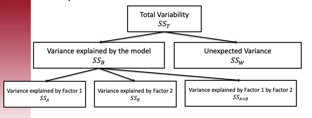
  • When we have factors influencing the outcome, the total variability can be decomposed as follows:

Sources of variability: Total variance can be decomposed into between-group and within-group variance

F-statistics

• Core idea: Comparing the variances between groups and within groups to ascertain if the means of different groups are significantly different from each other.

• Logic: If the between-group variance (due to systematic differences caused by the independent variable) is significantly greater than the within-group variance (attributable to random error), the observed differences between group means are likely not due to chance.

• F-statistics formula for one-way ANOVA:

  \[ F_{obs} = \frac{SS_{between}/df_{between}}{SS_{within}/df_{within}} \]

  • Degrees of freedom: \(df_{between}\) = 3 (groups) - 1 = 2, \(df_{within}\) = 16 (samples) - 3 (groups) = 13
  • \(SS_{between}\) = \(\sum n_j(\bar{Y}_j - \bar{Y})^2\) = 43.75
    • Variability in the differences between groups (weighted by group sample size)
  • \(SS_{within}\) = \(\sum_{j=1}^{3} \sum_{i=1}^{n_j}(Y_{ij}-\bar{Y}_j)^2\) = 14.00; where \(Y_{ij}\) is individual \(i\)’s score in group \(j\)
    • Random error within groups—individuals differ in attitudes for unknown reasons

Step 4: Conduct a hypothesis testing

• In addition to the comparison of the critical value and the observed value of the test statistics, we can also compare the alpha and the p-value:

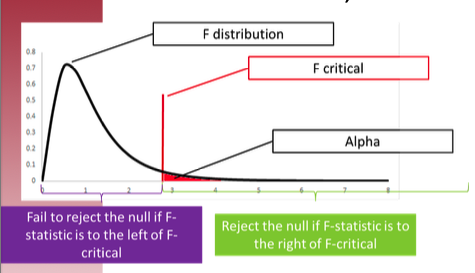
F-distribution showing rejection regions for different alpha levels

• We determine \(F_{crit}\) by setting \(\alpha\) value.
  • \(\alpha\) = (acceptable) type I error rate = probability that we wrongly reject \(H_0\) when \(H_0\) is true
• From the data, we obtain \(F_{obs}\) with p-value.
  • p-value = probability of datasets having F-statistics larger than \(F_{obs}\)
• If the F statistic from the data (\(F_{obs}\)) is larger than \(F_{critical}\), then you are in the rejection region and can reject \(H_0\) and accept \(H_A\) with \((1-\alpha)\) level of confidence.
• If the p-value obtained from the ANOVA is less than \(\alpha\), then reject \(H_0\) and accept \(H_A\) with \((1-\alpha)\) level of confidence.

Step 5: Results Report

A one-way ANOVA was conducted to compare the level of concern for tax reform among three political groups: Democrats, Republicans, and Independents. There was a significant effect of political affiliation on tax reform concern at the \(p < .001\) level for the three conditions [\(F(2, 13) = 20.31\), \(p < .001\)]. This result indicates significant differences in attitudes toward tax reform among the groups.

Limitation of ANOVA

Note: Relationship Between P-values and Type I Error

1. P-values: The probability of observing data as extreme as, or more extreme than, the data observed under the assumption that the null hypothesis is true.

   • The lower the p-value, the less likely we would see the observed data given the null hypothesis is true

   • Question: Given that we already have the observed data, does a lower p-value mean the null hypothesis is unlikely to be true?

   • Answer: No. \(P(\text{observed data} | H_0 = \text{true}) \neq P(H_0 = \text{true} | \text{observed data})\). P-values are often misconstrued as the probability that the null hypothesis is true given the observed data. However, this interpretation is incorrect.

2. Type I error, also known as a “false positive,” occurs when the null hypothesis is incorrectly rejected when it is, in fact, true.

3. The alpha level \(\alpha\) set before conducting a test (commonly \(\alpha = 0.05\)) defines the cutoff point for the p-value below which the null hypothesis will be rejected.

   • A p-value less than the alpha level suggests a low probability that the observed data would occur if the null hypothesis were true. Consequently, rejecting the null hypothesis in this context implies there is a statistically significant difference likely not due to random chance.

   • If you set up a high alpha level (0.1), you are more likely to have p-value lower than alpha, which means you are more likely reject the null hypothesis that may be true, which means you may make Type 1 error.

   • If you set up a low alpha level (0.001), you are less likely to have p-value lower than alpha, which means you are more likely retain the null hypothesis that may be false, which means you may make Type 2 error.

Note: Limitations of p-values

Relying solely on p-values to reject the null hypothesis can be problematic for several reasons:

• Binary Decision Making: The use of a threshold (e.g., \(\alpha = 0.05\)) to determine whether to reject the null hypothesis reduces the complexity of the data to a binary decision. This can oversimplify the interpretation and overlook nuances in the data.

  • Alternatives: Confidence intervals, Bayesian statistics (reporting posterior distributions)

• Neglect of Effect Size: P-values do not convey the size or practical importance of an effect. A very small effect can produce a small p-value if the sample size is large enough, leading to rejection of the null hypothesis even when the effect may not be practically significant.

  • Solution: Report effect sizes that are independent of sample size

• Probability of Extremes Under the Null: Since p-values quantify the extremeness of the observed data under the null hypothesis, they do not address whether similarly extreme data could also occur under alternative hypotheses. This can lead to an overemphasis on the null hypothesis and potentially disregard other plausible explanations for the data.

  • Solution: Explore theory, find alternative explanations, try varied models

A short quiz

Google form link

2 Example 2: the Effect of Sleep on Academic Performance (Simulation)

Background

• A study investigates the effect of different sleep durations on the academic performance of university students. Three groups are defined based on nightly sleep duration: Less than 6 hours, 6 to 8 hours, and more than 8 hours.

• We can simulate the data

# Set seed for reproducibility
set.seed(42)

# Generate data for three sleep groups
less_than_6_hours <- rnorm(30, mean = 65, sd = 10)
six_to_eight_hours <- rnorm(50, mean = 75, sd = 8)
more_than_8_hours <- rnorm(20, mean = 78, sd = 7)

# Combine data into a single data frame
sleep_data <- data.frame(
  Sleep_Group = factor(c(rep("<6 hours", 30), rep("6-8 hours", 50), rep(">8 hours", 20))),
  Exam_Score = c(less_than_6_hours, six_to_eight_hours, more_than_8_hours)
)

# View the first few rows of the dataset
head(sleep_data)

  Sleep_Group Exam_Score
1    <6 hours   78.70958
2    <6 hours   59.35302
3    <6 hours   68.63128
4    <6 hours   71.32863
5    <6 hours   69.04268
6    <6 hours   63.93875

## There are two columns: (1) Sleep_Group (Group variable, IV) (2) Exam_Score (Outcome, DV)
mod <- lm(Exam_Score ~ Sleep_Group, data = sleep_data)
mod_aov <- aov(mod)
summary(mod_aov) # F-value = 14.15, p < .05

            Df Sum Sq Mean Sq F value   Pr(>F)    
Sleep_Group  2   2411  1205.4   14.15 4.06e-06 ***
Residuals   97   8264    85.2                     
---
Signif. codes:  0 '***' 0.001 '**' 0.01 '*' 0.05 '.' 0.1 ' ' 1

Descriptive Statistics

• Groups:

  • Less than 6 hours: 30 students

  • 6 to 8 hours: 50 students

  • More than 8 hours: 20 students

• Performance Metric: Average exam scores out of 100.

  • Less than 6 hours: Mean = 65, SD = 10

  • 6 to 8 hours: Mean = 75, SD = 8

  • More than 8 hours: Mean = 78, SD = 7

Your Turn:

F-test

• Analysis: One-way ANOVA was conducted to compare the average exam scores among the three groups.

• Results: \(F_{observed}\) = [Calculate from your analysis], \(p\) = [Report p-value]

Interpretation

• Alpha Level: \(\alpha = 0.05\)

• P-value Interpretation: Compare your p-value to alpha and interpret the result

• Conclusion: Based on the results, what can you conclude about the effect of sleep duration on academic performance?

Homework 1

Due on next Tuesday Noon. Here is the google form link.