Lecture 05: Maximum Likelihood Estimation and Generalized Univariate Models

Today’s Class

Review last class - Random variables and their distribution
Self practice and self exercise using AI tutor
Graduate Certificate in Educational Statistics and Research Methods
I delayed Homework 2 to Week 11.
Maximum Likelihood Estimation
- The basics
- ML-based Test (Likelihood ratio test, Wald test, Information criteria)
- MLEs for GLMs

Graduate Certificate in ESRM

If you take this class, you already finish 25% or more in getting the graduate certificate.
You may waive the core courses if you take similar class, please consult Dr. Wenjuo Lo (wlo@uark.edu) for more details of the requirement.

AI tutor: self practice and self exercise

Self practice: Example Conversation
AI assignment: Interactive assignment

Today’s Example Data #1

To use the class example data, type in following R code: pak::pak("JihongZ/ESRM64503", upgrade = TRUE) or devtools::install_github("JihongZ/ESRM64503", upgrade = "always") to upgrade ESRM64503 package

Data Information

Purpose: imagine an employer is looking to hire employees for a job where IQ is important
- We will only use 5 observations so as to show the math behind the estimation calculations
The employer collects two variables:
- Predictor: IQ scores (labelled as iq)
- Outcome: Job performance (labelled as perf)

Descriptive Statistics

# pak::pak("JihongZ/ESRM64503", upgrade = TRUE)
library(ESRM64503)
library(tidyverse)

#data for class example
dat <- dataIQ |> 
  mutate(ID = 1:5) |> 
  rename(IQ = iq, Performance = perf) |> 
  relocate(ID)

dat

ID	Performance	IQ
1	10	112
2	12	113
3	14	115
4	16	118
5	12	114

dat |> 
  summarise(
    across(c(Performance, IQ), list(Mean = mean, SD = sd))
  ) |> 
  t() |> 
  as.data.frame() |> 
  rownames_to_column(var = "Variable") |> 
  separate(Variable, into = c("Variable", "Stat"), sep = "_") |> 
  pivot_wider(names_from = "Stat", values_from = "V1")

# A tibble: 2 × 3
  Variable     Mean    SD
  <chr>       <dbl> <dbl>
1 Performance  12.8  2.28
2 IQ          114.   2.30

dat |> 
  select(IQ, Performance) |> 
  cov() |> 
  as.data.frame() |> 
  rownames_to_column("Covariance Matrix")

  Covariance Matrix  IQ Performance
1                IQ 5.3         5.1
2       Performance 5.1         5.2

How Estimation Works (More or Less)

We need models to test the hypothesis, while models need estimation method to provide estimates of effect size.

Most estimation routines do one of three things:

Minimize Something: Typically found with names that have “least” in the title. Forms of least squares include “Generalized”, “Ordinary”, “Weighted”, “Diagonally Weighted”, “WLSMV”, and “Iteratively Reweighted.” Typically the estimator of last resort…
Maximize Something: Typically found with names that have “maximum” in the title. Forms include “Maximum likelihood”, “ML”, “Residual Maximum Likelihood” (REML), “Robust ML”. Typically the gold standard of estimators
Use Simulation to Sample from Something: more recent advances in simulation use resampling techniques. Names include “Bayesian Markov Chain Monte Carlo”, “Gibbs Sampling”, “Metropolis Hastings”, “Metropolis Algorithm”, and “Monte Carlo”. Used for complex models where ML is not available or for methods where prior values are needed.

Note

Loss function in Machine Learning belong to 1st type
lm use QR algorithm, which is one of methods for Ordinary Least Square (OLS) Estimation
Question: Maximum Likelihood Estimation belongs to 2nd type

Note: the estimates of regression coefficients provided by lm are using the OLS estimation method.

summary(lm(perf ~ iq, data = dataIQ))


Call:
lm(formula = perf ~ iq, data = dataIQ)

Residuals:
      1       2       3       4       5 
-0.4906  0.5472  0.6226 -0.2642 -0.4151 

Coefficients:
            Estimate Std. Error t value Pr(>|t|)   
(Intercept) -97.2830    15.5176  -6.269  0.00819 **
iq            0.9623     0.1356   7.095  0.00576 **
---
Signif. codes:  0 '***' 0.001 '**' 0.01 '*' 0.05 '.' 0.1 ' ' 1

Residual standard error: 0.6244 on 3 degrees of freedom
Multiple R-squared:  0.9438,    Adjusted R-squared:  0.925 
F-statistic: 50.34 on 1 and 3 DF,  p-value: 0.005759

Ordinary Least Square (OLS): Minimize Something

Definition and Core Concept

Ordinary Least Square (OLS) is an estimation method that finds the “best-fitting” line through data points by minimizing the sum of squared residuals
Key Idea: Among all possible lines, OLS chooses the one that makes the total squared distance between observed values and predicted values as small as possible

\text{Minimize: } \sum_{i=1}^{n} (y_i - \hat{y}_i)^2 = \sum_{i=1}^{n} (y_i - (\beta_0 + \beta_1 x_i))^2
Residual: The difference between observed value and predicted value: e_i = y_i - \hat{y}_i

Why “Least Squares”?

Alternative approaches could minimize:
- Sum of absolute deviations: \sum |y_i - \hat{y}_i| (less common)
- Sum of squared deviations: \sum (y_i - \hat{y}_i)^2 ← OLS choice
Advantages of squaring:
1. Mathematical tractability: Has closed-form solution using calculus
2. Penalizes large errors more: (-3)^2 = 9 vs (-1)^2 = 1
3. Eliminates sign issues: Both positive and negative residuals contribute positively

Mathematical Foundation

For simple linear regression y = \beta_0 + \beta_1 x + e, OLS estimates are:

\hat{\beta}_1 = \frac{\sum_{i=1}^{n}(x_i - \bar{x})(y_i - \bar{y})}{\sum_{i=1}^{n}(x_i - \bar{x})^2} = \frac{Cov(x,y)}{Var(x)}

\hat{\beta}_0 = \bar{y} - \hat{\beta}_1\bar{x}

OLS Visualization with Our Data

⌘+C

library(ggplot2)

# Calculate OLS estimates manually
x <- dat$IQ
y <- dat$Performance
n <- length(x)
x_mean <- mean(x)
y_mean <- mean(y)

# Calculate slope and intercept
beta1_hat <- sum((x - x_mean) * (y - y_mean)) / sum((x - x_mean)^2)
beta0_hat <- y_mean - beta1_hat * x_mean

# Create prediction line
x_range <- seq(min(x) - 5, max(x) + 5, length.out = 100)
y_pred <- beta0_hat + beta1_hat * x_range

# Create the plot
ggplot(dat, aes(x = IQ, y = Performance)) +
  geom_point(size = 3, color = "tomato", alpha = 0.8) +
  geom_line(data = data.frame(x = x_range, y = y_pred),
            aes(x = x, y = y), color = "royalblue", linewidth = 1.2) +
  geom_segment(aes(xend = IQ, yend = beta0_hat + beta1_hat * IQ),
               color = "gray40", linetype = "dashed", alpha = 0.7) +
  labs(title = "OLS Regression: Minimizing Sum of Squared Residuals",
       subtitle = paste0("ŷ = ", round(beta0_hat, 2), " + ", round(beta1_hat, 4), "x"),
       x = "IQ", y = "Performance") +
  theme_minimal() +
  annotate("text", x = min(x), y = max(y),
           label = paste0("Sum of Squared Residuals = ",
                         round(sum((y - (beta0_hat + beta1_hat * x))^2), 3)),
           hjust = 0, vjust = 1, color = "darkred", size = 4)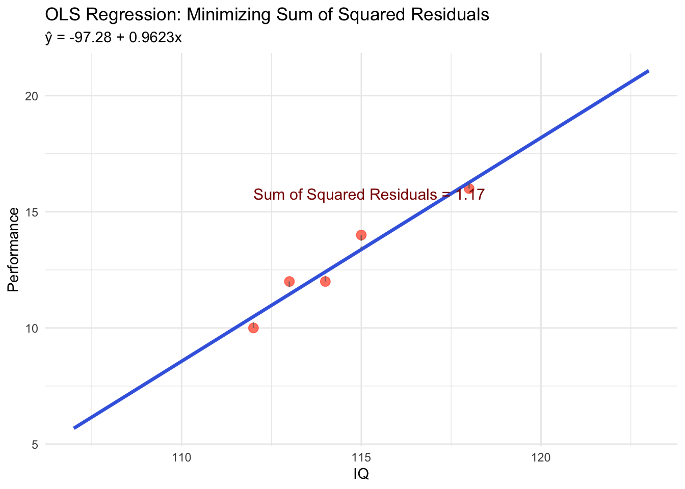

Comparison: OLS vs. Other Possible Lines

⌘+C

# Create several alternative lines for comparison
alternative_lines <- data.frame(
  Method = c("OLS (Optimal)", "Steeper Slope", "Flatter Slope", "Different Intercept"),
  Intercept = c(beta0_hat, beta0_hat - 5, beta0_hat + 3, beta0_hat + 10),
  Slope = c(beta1_hat, beta1_hat + 0.05, beta1_hat - 0.03, beta1_hat),
  Color = c("royalblue", "red", "orange", "purple")
)

# Calculate SSR for each line
alternative_lines$SSR <- sapply(1:nrow(alternative_lines), function(i) {
  pred <- alternative_lines$Intercept[i] + alternative_lines$Slope[i] * x
  sum((y - pred)^2)
})

# Create comparison plot
p <- ggplot(dat, aes(x = IQ, y = Performance)) +
  geom_point(size = 3, color = "black", alpha = 0.8)

# Add each line
for(i in 1:nrow(alternative_lines)) {
  line_data <- data.frame(
    x = x_range,
    y = alternative_lines$Intercept[i] + alternative_lines$Slope[i] * x_range
  )
  p <- p + geom_line(data = line_data, aes(x = x, y = y),
                     color = alternative_lines$Color[i], linewidth = 1.2)
}

p + labs(title = "OLS vs. Alternative Lines: Why OLS is Optimal",
         subtitle = "OLS minimizes the sum of squared residuals",
         x = "IQ", y = "Performance") +
  theme_minimal() +
  annotate("text", x = 105, y = 15,
           label = paste0("SSR Values:\n",
                         paste(alternative_lines$Method, ": ", round(alternative_lines$SSR, 2), collapse = "\n")),
           hjust = 0, vjust = 1, size = 3.5, color = "darkblue")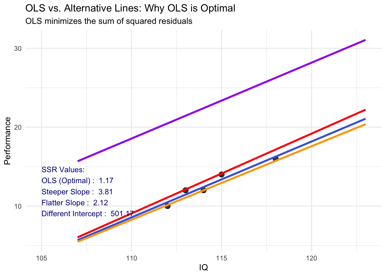

Maximum Likelihood Estimation (MLE): Maximize something

MLE has several good statistical properties that make it the mostly commonly used in multivariate statistics:
1. Asymptotic Consistency: as the sample size increases, the estimator converges in probability to parameters’ true values
2. Asymptotic Normality: as the sample size increases, the distribution of the estimator is normal (note: variance is given by “information” matrix)
3. Efficiency: No other estimator will have a smaller standard error

Terminology

Estimator: the algorithm that can get the estimates of parameters

Asymptotic: the properties that will occur when the sample size is sufficiently large

ML-based estimators: other variants of maximum likelihood like robust maximum likelihood, full information maximum likelihood

Maximum Likelihood: Estimates Based on Statistical Distributions

Maximum likelihood estimates come from statistical distributions - assumed distributions of data
- We will begin today with the univariate normal distribution but quickly move to other distributions
For a single random variable x, the univariate normal distribution is:

f(x) = \frac{1}{\sqrt{2\pi\color{tomato}{\sigma^2_x}}}\exp(-\frac{(x-\color{royalblue}{\mu_x})^2}{2\color{tomato}{\sigma^2_x}})
- Provides the height of the curve for a value of x, \mu_x, and \sigma^2
Last week we pretended we knew \mu_x and \sigma_x^2
- Today we will only know values of x and “guess” the parameters \mu_x and \sigma^2_x

Key Idea: Constructing a Likelihood Function

A likelihood function provides a value of a likelihood for a set of statistical parameters given observed data (denoted as L(\mu_x, \sigma^2_x|x))
If we observe the data (known) but do not know the mean and/or variance (unkown), then we call this the sample likelihood function
- The process of finding the values that maximizing the sample likelihood function is named Maximum Likelihood function
Likelihood functions is a probability density function (PDFs) of random variables that input observed data values
- Density functions are provided for each observation individually
- Each observation has its likelihood function.
- Mark this: We can get the “whole” likelihood of observed data by multiple all case-level likelihood.

Rather than providing the height of the curve of any value of x, it provides the likelihood for any possible values of parameters (i.e., \mu_x and/or \sigma^2_x)
- Goal of maximizing the sample likelihood function is to find optimal values of parameters
Assumption:
- All observed random variables follow certain probability density functions (i.e., x follows normal dis. and y follows Bernoulli dist.).
- The sample likelihood can be thought of as a joint distribution of all the observations, simultaneously
- In univariate statistics, observations are considered independent, so the joint likelihood for the sample is constructed through a product
To demonstrate, let’s consider the likelihood function for one observation that is used to estimate the mean and the variance of x

Example: One-Observation Likelihood function

Let’s assume:
- We just observed the first value of IQ (x = 112)
- Our initial guess is “the IQ comes from a normal distribution x \sim N(100, 5)”
- Our goal is to test whether this guess needed to be adjusted
Step 1: For this one observation, the likelihood function takes its assumed distribution and uses its PDF:

L(x_1=112|\mu_x = 100, \sigma^2_x = 5) = f(x_1, \mu_x, \sigma^2_x)= \frac{1}{\sqrt{2\pi*\color{tomato}{5}}}\exp(-\frac{(112-\color{royalblue}{100})^2}{2*\color{tomato}{5}})
- If you want to know the value of L(x_1), you can easily use R function dnorm(112, 100, sqrt(5)) , which gives your 9.94\times 10^{-8}.
- Because it is too small, typical we use log transformation of likelihood, which is called log likelihood. The value is -16.12

More observations: Multiplication of Likelihood

L(x_1 = 112|\mu_x = 100, \sigma^2_x = 5) can be interpreted as the Likelihood of first observation value being 112 given the underlying distribution is a normal distribution with mean as 100 and variance as 5.
Step 2: Then, for following observations, we can calculate their likelihood just similar to the first observation
- Now, we have L(x_2), L(x_3), …, L(x_N)
Step 3: Now, we multiple them together L(X|\mu_x=100, \sigma^2_x=5) =L(x_1)L(x_2)L(x_3)\cdots L(x_N), which represents the Likelihood of observed data existing given the underlying distribution is a normal distribution with mean as 100 and variance as 5.
Step 4: Again, we log transformed the likelihood to make the scale more easy to read: LL(X|\mu_x=100, \sigma^2_x=5)
Step 5: Finally, we change the value of parameters \mu_x and \sigma^2_x and calculate their LL (i.e., LL(X|\mu_x=101, \sigma^2_x=6))
- Eventually, we can get a 3-D density plot with x-axis and y-axis are varied values of \mu_x and \sigma^2_x; z-axis is their corresponding log-likelihood
- The set of \mu_x and \sigma^2_x which has the highest log-likelihood are the estimates of MLE

Visualization of MLE

The values of \mu_x and \sigma_x^2 that maximize L(\mu_x, \sigma^2_x|x) is \hat\mu_x = 114.4 and \hat{\sigma^2_x} = 4.2. We also know the mean of IQ is 114.2 and the variance of IQ is 5.3. Why the mean is same to estimate mu but variance is different? Answer: MLE is a biased estimator

⌘+C

library(plotly)
cal_LL <- function(x, mu, variance) {
   sum(log(sapply(x, \(x) dnorm(x, mean = mu, sd = sqrt(variance)))))
}
    
x <- seq(80, 150, 1)
y <- seq(3, 8, .5)
x_y <- expand.grid(x, y)
colnames(x_y) = c("mean", "variance")
dat2 <- x_y
dat2 <- dat2 |> 
    rowwise() |> 
    mutate(LL = cal_LL(x = dat$IQ, mu = mean, variance = variance)) |> 
    ungroup() |> 
    mutate(highlight = ifelse(LL == max(LL), TRUE, FALSE))

fig <- plot_ly(dat2, x =~mean, y = ~variance, z = ~LL, color = ~highlight, colors = c('#BF382A', '#0C4B8E'), alpha = 0.6)

fig <- fig %>% add_markers()

fig <- fig %>% layout(scene = list(xaxis = list(title = 'Weight'),

                     yaxis = list(title = 'Gross horsepower'),

                     zaxis = list(title = '1/4 mile time')))


fig

Maximizing the Log Likelihood Function

The process of finding the optimal estimates (i.e., \mu_x and \sigma_x^2) may be complicated for some models
- What we shown here was a grid search: trial-and-error process
For relatively simple functions, we can use calculus to find the maximum of a function mathematically
- Problem: not all functions can give closed-form solutions (i.e., one solvable equation) for location of the maximum
- Solution: use optimization algorithms of searching for parameter (i.e., Expectation-Maximum algorithm, Newton-Raphson algorithm, Coordinate Descent algorithm)

Estimate Regression Coefficients

Y \sim N(\beta_0+\beta_1X, \sigma_e)

f(y) = \frac{1}{\sqrt{2\pi\color{tomato}{\sigma^2_e}}}\exp(-\frac{(y-\color{royalblue}{(\beta_0+\beta_1x)})^2}{2\color{tomato}{\sigma^2_e}})

Both y and x are included in data, so we can create the likelihood function for \beta_0, \beta_1, and \sigma^2_e, just similar to what we did to \mu_x and \sigma^2_x.

For one data point with iq = 112 and perf = 10, we first assume \sigma^2_e = 1 and \beta_0 = 0

L(\beta_1=1 | \beta_0 = 0, \sigma^2_e = 1) = \frac{1}{\sqrt{2\pi*\color{tomato}{1}}}\exp(-\frac{(112-\color{royalblue}{(0+1*112)})^2}{2*\color{tomato}{1}})

We can iterate over different value of \beta_1 to see which value has highest likelihood. The move on to \beta_0 given fixed value of \beta_1 and \sigma^2_e

Note

Note that in modern software, the number of parameters is large. The iteration process over \beta_1 and other parameters is speeded up via optimization method (i.e., first derivation).

Useful Properties of MLEs

Next, we demonstrate three useful properties of MLEs (not just for GLMs)
- Likelihood ratio (aka Deviance) tests
- Wald tests
- Information criteria
To do so, we will consider our example where we wish to predict job performance from IQ (but will now center IQ at is mean of 11.4)
We will estimate two models, both used to demonstrate how ML estimation differs slightly from LS estimation for GLMs
- Empty model predicting just performance: Y_p = \beta_0 + e_p
- Model where mean centered IQ predicts performance:
  
  Y_p =\beta_0+\beta_1(IQ - 114.4) + e_p

`nlme` package: Maximum Likelihood

lm() function in previous lectures uses ordinary least square (OLS) for estimation; To use ML, we can use nlme pakage
nlme is a R package for nonlinear mixed-effects model

gls() for the empty model predicting performance:

library(nlme)
# empty model predicting performance
1model01 <- gls(iq~1, data = dataIQ, method = "ML")
summary(model01)

1: make sure method argument is set to “ML”

Generalized least squares fit by maximum likelihood
  Model: iq ~ 1 
  Data: dataIQ 
      AIC      BIC   logLik
  25.4122 24.63108 -10.7061

Coefficients:
            Value Std.Error  t-value p-value
(Intercept) 114.4  1.029563 111.1151       0

Standardized residuals:
         1          2          3          4          5 
-1.1655430 -0.6799001  0.2913858  1.7483146 -0.1942572 
attr(,"std")
[1] 2.059126 2.059126 2.059126 2.059126 2.059126
attr(,"label")
[1] "Standardized residuals"

Residual standard error: 2.059126 
Degrees of freedom: 5 total; 4 residual

`gls()`: Residuals, Information Criteria

gls function will return an object of class “gls” representing the linear model fit
- Generic functions like print, plot, and summary can be used to show the results of the model fitting
- The functions resid, coef, fitted can be used to extract residuals, coefficients, and predicted values

1as.numeric(resid(model01))
2attr(resid(model01), "std")

1: Residuals: Deviation of observed value (IQ) from predicted value (IQ)
2: Residual standard deviation (standard error)

[1] -2.4 -1.4  0.6  3.6 -0.4
[1] 2.059126 2.059126 2.059126 2.059126 2.059126

Same results can be found in summary function’s output as well

Residual standard error: 2.059126 Degrees of freedom: 5 total; 4 residual

Note that R found the same estimate of \sigma^2_e (residual variance) as 2.059126^2 = 4.24
The Information Criteria section of summary shows statistics that can be used for model comparisons

AIC(model01)
BIC(model01)
logLik(model01)

[1] 25.4122
[1] 24.63108
'log Lik.' -10.7061 (df=2)

`gls`: Fixed Effects

The coefficients (also referred to as fixed effects) are where the estimated regression slopes are listed

1summary(model01)$tTable

1: You can use str(summary(model01)) to check how many components the output contains

            Value Std.Error  t-value     p-value
(Intercept) 114.4  1.029563 111.1151 3.93391e-08

Here, \beta_0^{IQ}=\mu_x= 114.4, which is exactly same as the results of our manually coded ML algorithm
Difference from OLS we learnt last week:
- Traditional ANOVA table with Sums of Squares (SS), Mean Squares (MS) are no longer listed
- The Mean Square Error is no longer the estimate of \sigma^2_e: this comes directly from the model estimation algorithm itself.
- The tradition R^2 change test (F test) also changes under ML estimation

anova(model01)

Denom. DF: 4 
            numDF  F-value p-value
(Intercept)     1 12346.57  <.0001

anova(lm(iq~1, data = dataIQ))

Analysis of Variance Table

Response: iq
          Df Sum Sq Mean Sq F value Pr(>F)
Residuals  4   21.2     5.3

Useful Properties of MLEs

Next, we demonstrate three useful properties of MLEs (not just for GLMs)
- Likelihood ratio (aka Deviance) tests
- Wald tests
- Information criteria
To do so, we will consider our example where we wish to predict job performance from IQ (but will now center IQ at its mean of 114.4)
We will estimate two models, both used to demonstrate how ML estimation differs slightly from LS estimation for GLMs
- Empty model predicting just performance: Y_p = \beta_0 + e_p
- Model where mean centered IQ predicts performance: Y_p = \beta_0 + \beta_1 (IQ - 114.4) + e_p

Model Estimations

Model 02: The empty model predicting performance

# empty model predicting performance
model02 = gls(perf ~ 1, data = dataIQ, method = "ML")
summary(model02)$tTable |> show_table()

	Value	Std.Error	t-value	p-value
(Intercept)	12.8	1.019804	12.55143	0.0002319

Model 03: The conditional model where mean centered IQ predicts performance

# centering IQ at mean of 114.4
dataIQ$iq_114 <- dataIQ$iq - mean(dataIQ$iq)

# conditional model with cented IQ as predictor
model03a = gls(perf ~ iq_114, data = dataIQ, method = "ML")
summary(model03a)$tTable |> show_table()

	Value	Std.Error	t-value	p-value
(Intercept)	12.8000000	0.2792623	45.835048	0.0000229
iq_114	0.9622642	0.1356218	7.095205	0.0057592

Model Comparison

Research Questions in comparing between the two models that can be answered using ML:
- Q1: How do we test the hypothesis that IQ predicts performance?
  - Likelihood ratio tests (LRT; can be multiple parameters)
  - Wald tests (usually for one parameters)
- Q2: If IQ does significantly predict performance, what percentage of variance in performance does it account for?
  - Relative change in \sigma^2_e from empty model to conditional model

Method 1: Likelihood Ratio (Deviance) Tests

The likelihood value from MLEs can help to statistically test competing models assuming the models are nested
Likelihood ratio tests take the ratio of the likelihood for two models and use it as a test statistic
Using log-likelihoods, the ratio becomes a difference
- The test is sometimes called a deviance test \log{\frac{A}{B}} = \log{A} - \log{B}
D = - 2\Delta = -2 \times (\log{L_{H0}}-\log{L_{H1}})
- LRT is tested against a Chi-square distribution with degrees of freedom equal to the difference in number of parameters

Apply LRT to answer research question 1

Q1: How do we test the hypothesis that IQ predicts performance?
- Step 1: This can be translated to statistical language as: “test the null hypothesis that \beta_1 is squal to zero”:
H_0: \beta_1 = 0

H_1: \beta_1 \neq 0
- Step 2: The degree of freedom (df) of LRT is one parameter: the difference in number of parameters between the empty model and the conditional model
K_{M3a} - K_{M2} = 3 - 2 = 1

Note that the empty model (Model 2) has two parameters: \beta_0 and \sigma^2_e and the conditional model (Model 3a) has three parameters: \beta_0, \beta_1 and \sigma^2_e
- Step 3: estimate the -2*log-likelihood for both models and compute Deviance (D)
```
(neg2LL_model02 <-  logLik(model02))
```
```
'log Lik.' -10.65848 (df=2)
```
```
(neg2LL_model03a <- logLik(model03a))
```
```
'log Lik.' -3.463204 (df=3)
```
```
(D = as.numeric(-2 *(neg2LL_model02 - neg2LL_model03a)))
```
```
[1] 14.39055
```
- Step 4: calculate p-value from Chi-square distribution with 1 DF
```
pchisq(q = D, df = 1, lower.tail = FALSE)
```
```
[1] 0.0001485457
```
Alternatively, we can use anova to get the results of LRT more easily.
```
1anova(model02, model03a)
```
1

Using anova with two models in the parenthesis to autimatically calculate Likelihood ratio test (LRT) for you
```
         Model df      AIC      BIC     logLik   Test  L.Ratio p-value
model02      1  2 25.31696 24.53584 -10.658480                        
model03a     2  3 12.92641 11.75472  -3.463204 1 vs 2 14.39055   1e-04
```
- Inference: the regression slope for IQ was significantly different from zero - we prefer our alternative model to the null model
- Interpretation: IQ significantly predicts performance

Apply Wald Tests to Answer Question 1 (Usually 1 DF tests in Software)

For each parameter \theta, we can form the Wald statistic:

\omega = \frac{\theta_{MLE} - \theta_0}{SE(\theta_{MLE})}

Typically \theta_0 = 0
As N gets large (goes to infinity), the Wald statistic converges to a standard normal distribution
If we divide each parameter by its standard error, we can compute the two-tailed p-value from the standard normal distribution
- Exception: bounded parameters can have issues (variances)
We can further add that variances are estimated, switching this standard normal distribution to a t distribution (R does this for us for some packages)

Student t’s distribution

Recall that (in your introduction to statistics class) the degree of freedom of t-distribution follows:

df = N - p - 1 = 5-1-1 = 3 where N is the sample size (N = 5), p is the number of predictor (p = 1). For lower value of df, t value should be higher to have p-value smaller than alpha level as .05.

⌘+C

set.seed(1234)
x <- seq(-5, 5, .1)
dat <- data.frame(
  x = x,
  `t_dist_1` = dt(x, df = 1),
  `t_dist_2` = dt(x, df = 2),
  `t_dist_3` = dt(x, df = 3),
  `t_dist_4` = dt(x, df = 4),
  normality = dnorm(x)
) |> 
  pivot_longer(-x)
ggplot(dat) +
  geom_path(aes(x = x, y = value, color = name), linewidth = 1.2, alpha = .8) +
  geom_hline(yintercept = .05, linetype = "dashed", linewidth = 1.2) +
  labs(y = "Density", x = "t value", title = "Probability Density Function for Normal and T-statistics with varied DFs") +
  theme_classic() +
  scale_color_brewer(palette = "Set1",
                     labels = c("Normal Dist.", 
                                "Student's t Dist with df = 1",
                                "Student's t Dist with df = 2",
                                "Student's t Dist with df = 3",
                                "Student's t Dist with df = 4"),
                     name = "")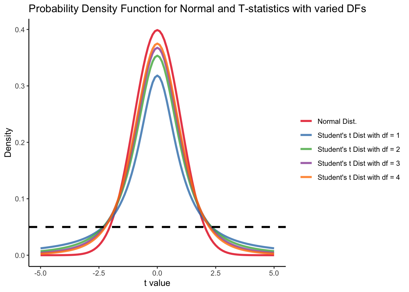

F Distribution

The degree of freedom of F distribution are df_1 = 1 and df_2 = N - p = 5 - 2 = 3. The probability distribution of F statistics can be achieved using pf in R. When we have larger sample size or less parameters to be estimated, same F-statistic will be more likely to be significant. (We have more statistical power!) Power analysis will tell us what is the minimum sample sample required to make one reasonable statistic significant.

⌘+C

set.seed(1234)
x <- seq(0, 10, .1)
dat <- data.frame(
  x = x,
  `F_dist_1` = pf(x, df1 = 1, df2 = 3, lower.tail = FALSE),
  `F_dist_2` = pf(x, df1 = 1, df2 = 10, lower.tail = FALSE),
  `F_dist_3` = pf(x, df1 = 1, df2 = 100, lower.tail = FALSE),
  `F_dist_4` = pf(x, df1 = 1, df2 = 1000, lower.tail = FALSE)
) |> 
  pivot_longer(-x)
ggplot(dat) +
  geom_path(aes(x = x, y = value, color = name), linewidth = 1.2, alpha = .8) +
  geom_hline(yintercept = .05, linetype = "dashed", linewidth = 1.2) +
  labs(y = "Probability", x = "F value", title = "Probability Function for F-statistics with varied DFs") +
  theme_classic() +
  scale_color_brewer(palette = "Set1",
                     labels = c(
                                "F Dist with df1 = 1, df2 = 3",
                                "F Dist with df1 = 1, df2 = 10",
                                "F Dist with df1 = 1, df2 = 100",
                                "F Dist with df1 = 1, df2 = 1000"),
                     name = "")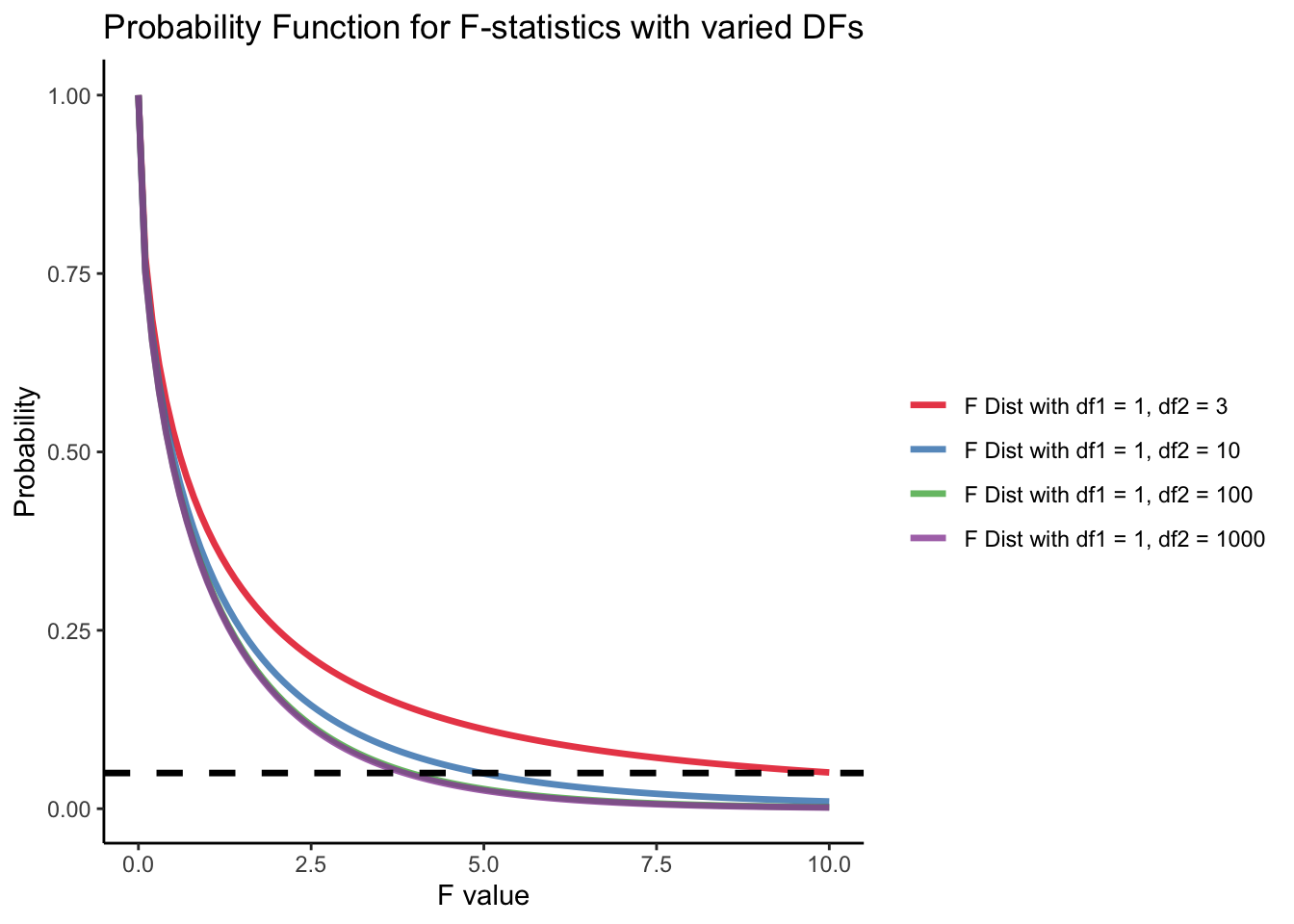

Wald test example

R provides the Wald test statistic for us from the summary()or anova() function:
One provides t-value, and the other provide F-value, but they have same p-values

summary(model03a)$tTable |> show_table()

	Value	Std.Error	t-value	p-value
(Intercept)	12.8000000	0.2792623	45.835048	0.0000229
iq_114	0.9622642	0.1356218	7.095205	0.0057592

anova(model03a) |> show_table()

	numDF	F-value	p-value
(Intercept)	1	2100.85161	0.0000229
iq_114	1	50.34194	0.0057592

Manual Calculation

\hat{t} = \frac{\hat{\beta}-0}{\text{SE}(\hat{\beta})}

\hat{F} = \hat{t}^2

coef_table <- summary(model03a)$tTable
(t_value_beta1 <- ((coef_table[2, 1] - 0) / coef_table[2, 2]))

[1] 7.095205

(F_value_beta1 <- t_value_beta1^2)

[1] 50.34194

pt(t_value_beta1, 3, lower.tail = FALSE)*2 # p-value for two-tail t-test with df = 3

[1] 0.005759162

pf(F_value_beta1, 1, 3, lower.tail = FALSE) # p-value for f-statistic with df1=1 and df2=3

[1] 0.005759162

Here, the slope estimate has a t-test statistic value of 7.095 (p = 0.0057592), meaning we would reject our null hypothesis, indicating that the IQ can predict performance significant
Typically, Wald tests are used for one additional parameter
- Here, one parameter – slope of IQ

Method 2: Model Comparison with R^2

To compute an R^2, we use the ML estimates of \sigma^2_e:
- Empty model: \sigma^2_e = 4.160 (2.631)
- Conditional model: \sigma^2_e = 0.234 (0.145)

#  Residual variance for model02
1(model02$sigma^2 -> resid_var_model02)
# Residual variance for model03a
(model03a$sigma^2 -> resid_var_model03a)

1: use $sigma to extract standard errors

[1] 4.16
[1] 0.2339623

The R^2 for variance in performance accounted for by IQ is:

R^2 = \frac{4.160 - 0.234}{4.160} = .944 The model3a (IQ) can explain 94.4% unexplained variance by empty model.

Method 3: Information Criteria

Information criteria are statistics that help determine the relative fit of a model for non-nested models
- Comparison is fit-versus-parsimony
R reports a set of criteria (from conditional model)

anova(model02, model03a)

         Model df      AIC      BIC     logLik   Test  L.Ratio p-value
model02      1  2 25.31696 24.53584 -10.658480                        
model03a     2  3 12.92641 11.75472  -3.463204 1 vs 2 14.39055   1e-04

Each uses -2*log-likelihood as a base
Choice of IC is very arbitrary and depends on field
Best model is one with smallest value
Note: don’t use information criteria for nested models
- LRT/Deviance tests are more powerful

Practice Exercise: Model Comparison Methods

Now let’s practice what we learned! Try to complete the following exercises using the methods we discussed.

Setup: We have fitted two models to predict job performance from IQ: - Model A (Empty): perf ~ 1 - Model B (Conditional): perf ~ iq_114 (where iq_114 is centered IQ)

Your Tasks:

Likelihood Ratio Test (LRT):
- Calculate the deviance (D) manually using log-likelihoods
- Compute the p-value from Chi-square distribution
- Compare with anova() function results
R-squared Calculation:
- Extract residual variances from both models
- Calculate R² as the proportion of variance explained
- Interpret the result
Information Criteria:
- Extract AIC and BIC values for both models
- Determine which model is preferred by each criterion

Here are the complete solutions:

Task 1: Likelihood Ratio Test (LRT)

Task 2: R-squared Calculation

Task 3: Information Criteria

When We should use Which

We introduce LRT, Wald test, R^2, and information criteria
We typically always report R^2 (for explained variances) and Wald test (for single parameters).
Then, when we have multiple model to comparison, we need to decide on whether these models are nested:

If they are nested, we reported LRT statistics
If they are not nested, we choose one IC to report (AIC, BIC either one is good, reporting both is best)

How ML and Least square Estimation of GLMs differ

You may have recognized that the ML and the LS estimates of the fixed effects were identical
And for these models, they will be
Where they differ is in their estimate of the residual variance \sigma^2_e:
- From least squares (MSE): \sigma^2_e = 0.390 (no SE)
- From ML (model parameter): \sigma^2_e = 0.234 (no SE in R)
The ML version uses a bias estimate of \sigma^2_e (it is too small)
Because \sigma^2_e plays a role in all SEs, the Wald tests differed from LS and ML
Don’t be troubled by this. A fix will come in a few weeks …
- Hint: use method = “REML” rather than method = “ML” in gls()

Wrapping Up

This lecture was our firs pass at maximum likelihood estimation
The topics discussed today apply to all statistical models, not just GLMs
Maximum likelihood estimation of GLMs helps when the basic assumptions are obviously violated
- Independence of observations
- Homogeneous \sigma^2_e
- Conditional normality of Y (normality of error terms)

Today’s Class

Graduate Certificate in ESRM

AI tutor: self practice and self exercise

Today’s Example Data #1

Data Information

Descriptive Statistics

How Estimation Works (More or Less)

Ordinary Least Square (OLS): Minimize Something

Definition and Core Concept

Why “Least Squares”?

Mathematical Foundation

OLS Visualization with Our Data

Comparison: OLS vs. Other Possible Lines

Maximum Likelihood Estimation (MLE): Maximize something

Maximum Likelihood: Estimates Based on Statistical Distributions

Key Idea: Constructing a Likelihood Function

Example: One-Observation Likelihood function

More observations: Multiplication of Likelihood

Visualization of MLE

Maximizing the Log Likelihood Function

Estimate Regression Coefficients

Useful Properties of MLEs

nlme package: Maximum Likelihood

gls(): Residuals, Information Criteria

gls: Fixed Effects

Useful Properties of MLEs

Model Estimations

Model Comparison

Method 1: Likelihood Ratio (Deviance) Tests

Apply LRT to answer research question 1

Apply Wald Tests to Answer Question 1 (Usually 1 DF tests in Software)

Student t’s distribution

F Distribution

Wald test example

Manual Calculation

Method 2: Model Comparison with R^2

Method 3: Information Criteria

Practice Exercise: Model Comparison Methods

When We should use Which

How ML and Least square Estimation of GLMs differ

Wrapping Up

`nlme` package: Maximum Likelihood

`gls()`: Residuals, Information Criteria

`gls`: Fixed Effects