Prior distribution - belief / previous evidences of parameters
Posterior distribution - updated information of parameters given our data and model
Posterior predictive distribution - future / predicted data
What are the differences between Bayesian with Frequentist analysis?
prior distribution: Bayesian
hypothesis of fixed parameters: frequentist
estimation process: MCMC vs. Maximum likelihhood estimation (MLE) or ordinary least square (OLS)
posterior distribution vs. point estimates of parameters
credible interval (plausibility of the parameters having those values) vs. confidence interval (the proportion of infinite samples having the fixed parameters)
The Likelihood function \(P(X|p_1)\) follows Binomial distribution of 3 succuess out of 5 samples: \[P(X|p_1) = \prod_{i =1}^{N=5} p_1^{X_i}(1-p_1)^{X_i}
\\= (1-p_i) \cdot p_i \cdot (1-p_i) \cdot p_i \cdot p_i\]
Question here: WHY use Bernoulli (Binomial) Distribution (feat. Jacob Bernoulli, 1654-1705)?
My answer: Bernoulli dist. has nice statistical probability. “Nice” means making totally sense in normal life– a common belief. For example, the \(p_1\) value that maximizes the Bernoulli-based likelihood function is \(Mean(X)\), and the \(p_1\) values that minimizes the Bernoulli-based likelihood function is 0 or 1
Log-likelihood Function along “Parameter”
Assume each event is independent, the multiplication of the probabilities of each event is the “Likelihood”. Log transform of Likelihood is easier for further analysis.
\[
LL(p_1|\{0, 1, 0, 1, 1\})
\]
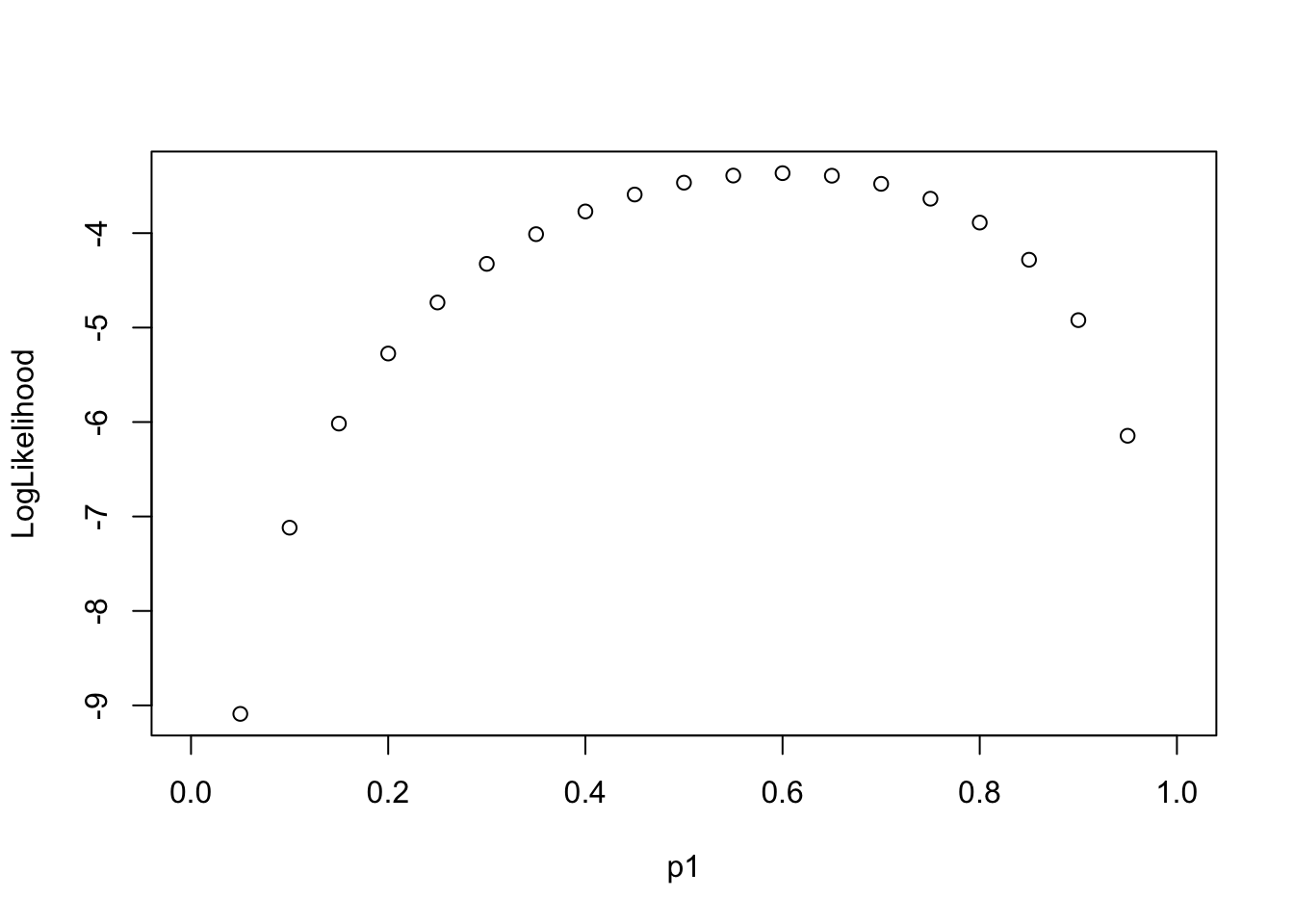
Goal: find the most possible p1 value (the probability of the event) so that the data {0, 1, 0, 1, 1} has the highest likelihood
## iterate over different plausible values of p1 ranging [0, 1]p1 =seq(0, 1, length.out =21) Likelihood = (p1)^3* (1-p1)^2LogLikelihood =log(Likelihood)plot(x = p1, y = LogLikelihood)
p1[which.max(Likelihood)] # p1 = 0.6 = 3 / 5
[1] 0.6
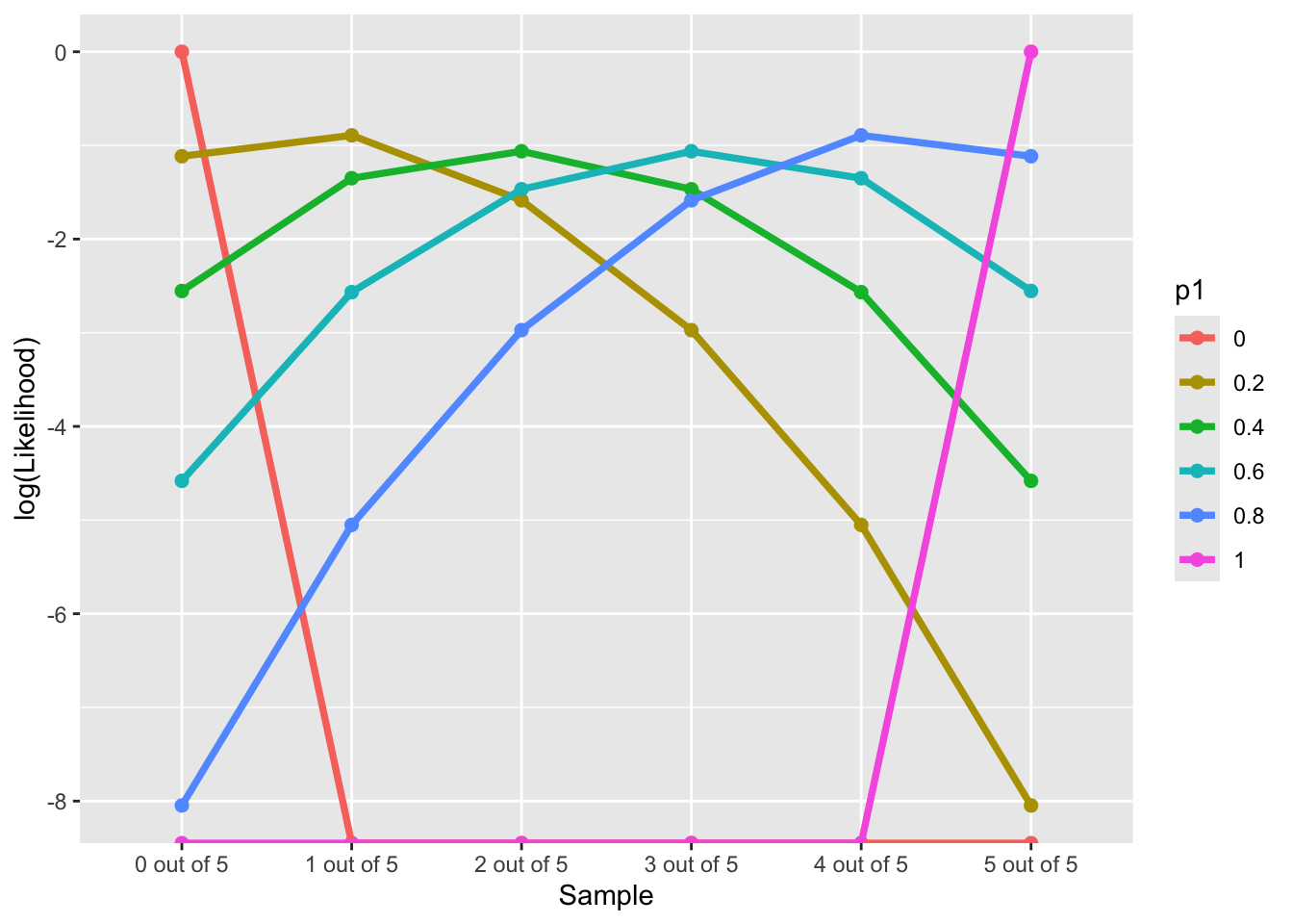
Log-likelihood Function along “Data”
\[
LL(Data|p_1 \in \{0, 0.2,0.4, 0.6, 0.8,1\})
\]
Code
library(tidyverse)p1 =c(0, 2, 4, 6, 8, 10) /10nTrails =5nSuccess =0:nTrailsLikelihood =sapply(p1, \(x) choose(nTrails,nSuccess)*(x)^nSuccess*(1-x)^(nTrails - nSuccess))Likelihood_forPlot <-as.data.frame(Likelihood)colnames(Likelihood_forPlot) <- p1Likelihood_forPlot$Sample =factor(paste0(nSuccess, " out of ", nTrails), levels =paste0(nSuccess, " out of ", nTrails))# plotLikelihood_forPlot %>%pivot_longer(-Sample, names_to ="p1") %>%mutate(`log(Likelihood)`=log(value)) %>%ggplot(aes(x = Sample, y =`log(Likelihood)`, color = p1)) +geom_point(size =2) +geom_path(aes(group=p1), size =1.3)
Step 2: Choose the Prior Distribution for \(p_1\)
We must now pick the prior distribution of \(p_1\):
\[
P(p_1)
\]
Compared to likelihood function, we have much more choices. Many distributions to choose from
To choose prior distribution, think about what we know about a “fair” die.
the probability of rolling a “1” is about \(\frac{1}{6}\)
the probabilities much higher/lower than \(\frac{1}{6}\) are very unlikely
Let’s consider a Beta distribution as the prior distribution of \(p_1\):
\[
p_1 \sim Beta(\alpha, \beta)
\]
or
\[
P(p_1) \equiv Beta(\alpha, \beta)
\]
The Beta Distribution
For parameters that range between 0 and 1, the beta distribution makes a good choice for prior distribution:
The Beta distribution has a mean of \(\frac{\alpha}{\alpha+\beta}\) and a mode of \(\frac{\alpha -1}{\alpha + \beta -2}\) for \(\alpha > 1\) & \(\beta > 1\); (fun fact: when \(\alpha\ \&\ \beta< 1\), pdf is U-shape, what that mean?)
\(\alpha\) and \(\beta\) are called hyperparameters of the parameter \(p_1\);
Hyperparameters are parameters of prior parameters ;
When \(\alpha = \beta = 1\), the distribution is uniform distribution;
To make sure \(P(p_1 = \frac{1}{6})\) is the largest, we can:
Many choices of prior distribution:
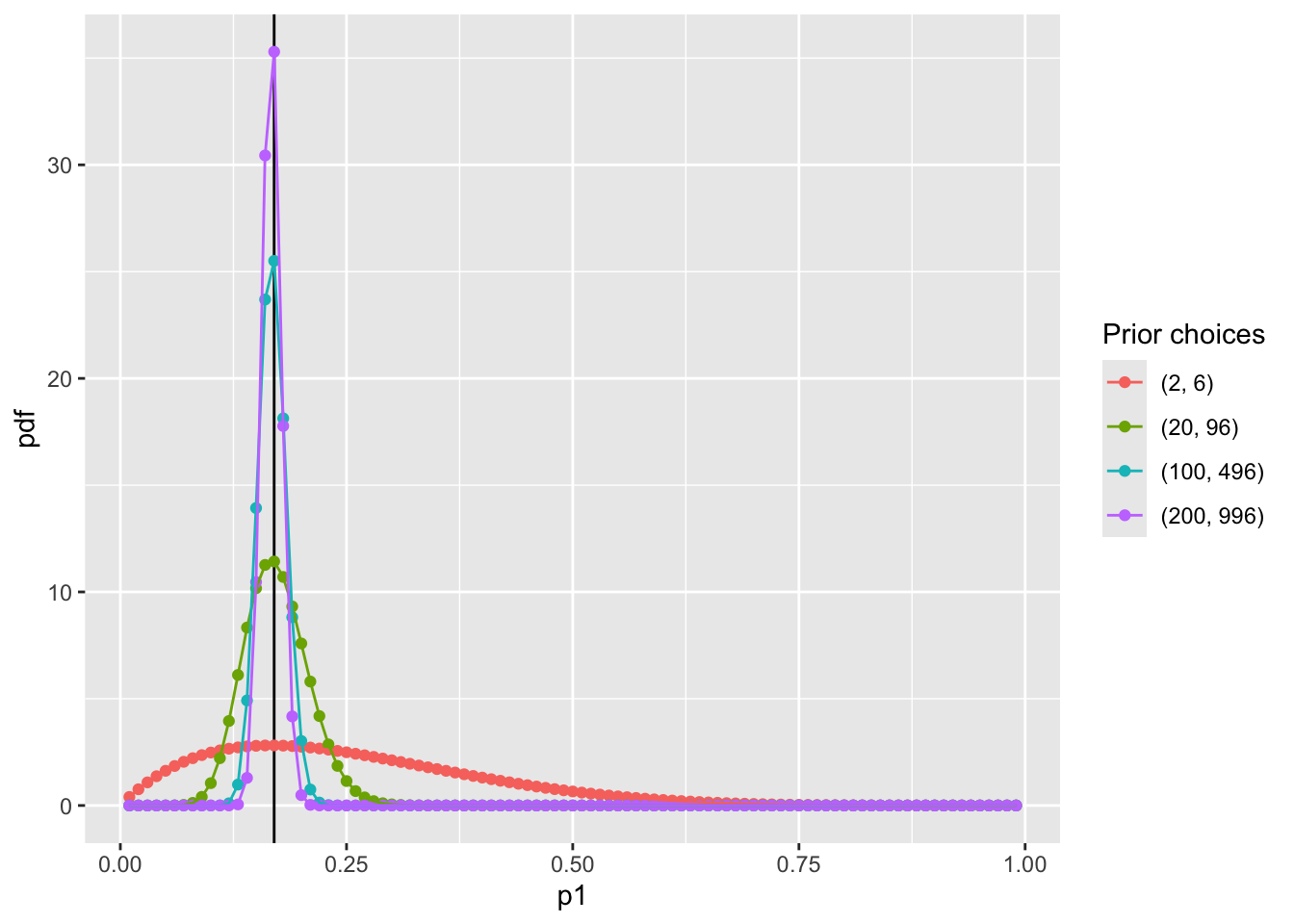
\(\alpha =2\) and \(\beta = 6\) has the same mode as \(\alpha = 100\) and \(\beta = 496\);
hint: when the relationship between \(\alpha\) and \(\eta\) follows \(\beta = 5\alpha - 4\)
The differences between choices is how strongly we feel in our beliefs
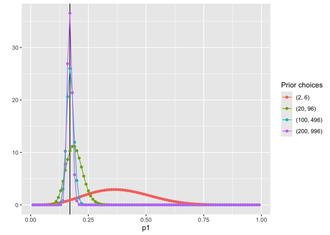
Visualize prior distribution \(P(p_1)\)
Code
dbeta <-function(p1, alpha, beta) {# probability density function PDF = ((p1)^(alpha-1)*(1-p1)^(beta-1)) /beta(alpha, beta)return(PDF)}condition <-data.frame(alpha =c(2, 20, 100, 200),beta =c(6, 96, 496, 996))pdf_bycond <- condition %>%nest_by(alpha, beta) %>%mutate(data =list(dbeta(p1 = (1:99)/100, alpha = alpha, beta = beta) ))## prepare data for plotting pdf by conditionspdf_forplot <-Reduce(cbind, pdf_bycond$data) %>%t() %>%as.data.frame() ## merge conditions togethercolnames(pdf_forplot) <- (1:99)/100# add p1 values as x-axispdf_forplot <- pdf_forplot %>%mutate(Alpha_Beta =c( # add alpha_beta conditions as colors"(2, 6)","(20, 96)","(100, 496)","(200, 996)" )) %>%pivot_longer(-Alpha_Beta, names_to ='p1', values_to ='pdf') %>%mutate(p1 =as.numeric(p1),Alpha_Beta =factor(Alpha_Beta,levels =unique(Alpha_Beta)))pdf_forplot %>%ggplot() +geom_vline(xintercept =0.17, col ="black") +geom_point(aes(x = p1, y = pdf, col = Alpha_Beta)) +geom_path(aes(x = p1, y = pdf, col = Alpha_Beta, group = Alpha_Beta)) +scale_color_discrete(name ="Prior choices")
Question: WHY NOT USE NORMAL DISTRIBUTION?
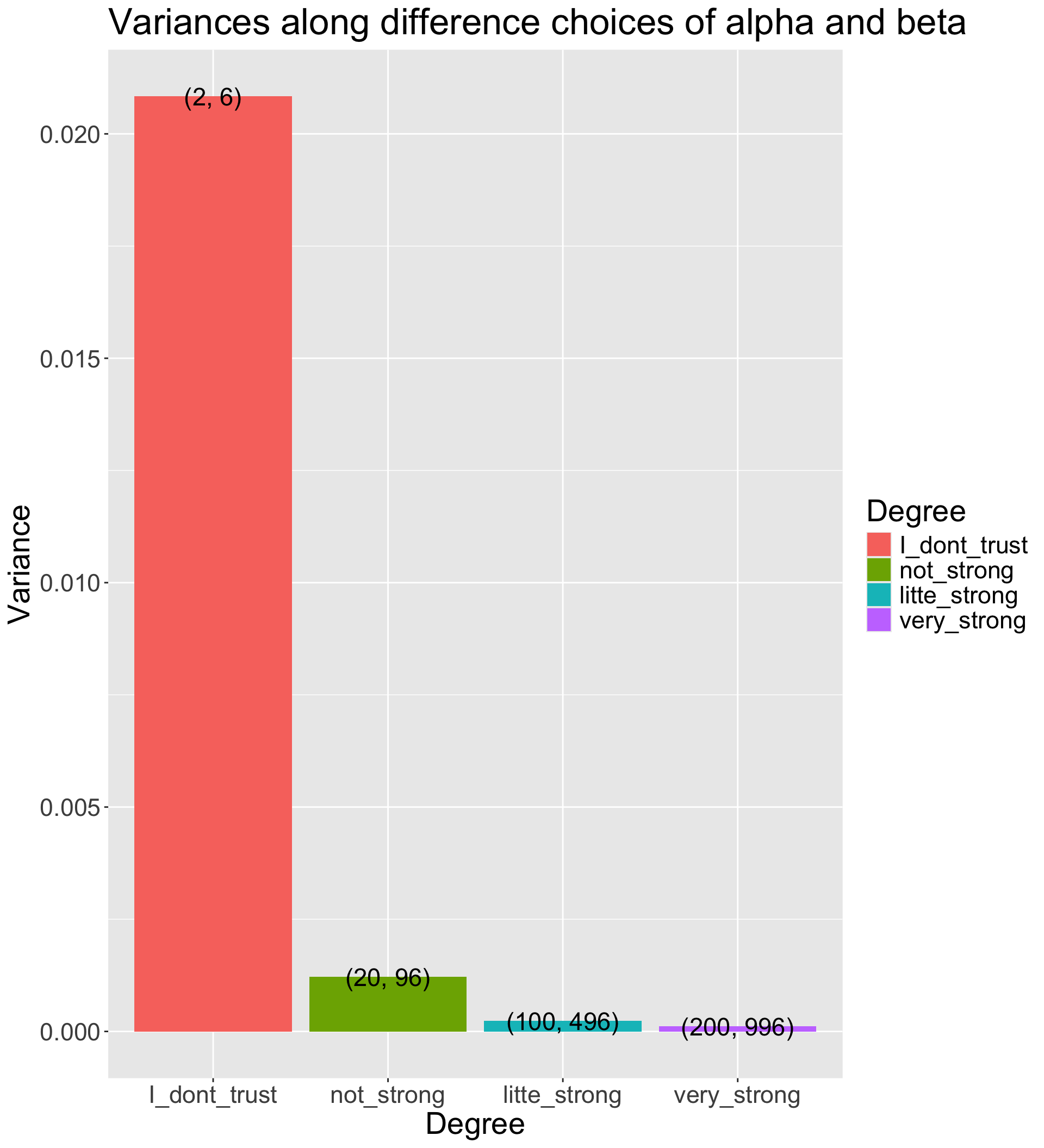
How strongly we believe in the prior
The Beta distribution has a variance of \(\frac{\alpha\beta}{(\alpha+\beta)^2 (\alpha + \beta + 1)}\)
The smaller prior variance means the prior is more informative
Informative priors are those that have relatively small variances
Uninformative priors are those that have relatively large variances
Suppose we have four sets of hyperparameters choices: (2,6);(20,96);(100,496);(200,996)
Code
# Function for variance of Beta distributionvarianceFun =function(alpha_beta){ alpha = alpha_beta[1] beta = alpha_beta[2]return((alpha * beta)/((alpha + beta)^2*(alpha + beta +1)))}# Multiple prior choices from uninformative to informativealpha_beta_choices =list(I_dont_trust =c(2, 6), not_strong =c(20, 96), litte_strong =c(100, 496), very_strong =c(200, 996))## Transform to data.frame for plotalpha_beta_variance_plot <-t(sapply(alpha_beta_choices, varianceFun)) %>%as.data.frame() %>%pivot_longer(everything(), names_to ="Degree", values_to ="Variance") %>%mutate(Degree =factor(Degree, levels =unique(Degree))) %>%mutate(Alpha_Beta =c("(2, 6)","(20, 96)","(100, 496)","(200, 996)" ))alpha_beta_variance_plot %>%ggplot(aes(x = Degree, y = Variance)) +geom_col(aes(fill = Degree)) +geom_text(aes(label = Alpha_Beta), size =6) +labs(title ="Variances along difference choices of alpha and beta") +theme(text =element_text(size =21))
Step 3: The Posterior Distribution
Choose a Beta distribution as the prior distribution of \(p_1\) is very convenient:
When combined with Bernoulli (Binomial) data likelihood, the posterior distribution (\(P(p_1|Data)\)) can be derived analytically
The posterior distribution is also a Beta distribution
\(\alpha' = \alpha + \sum_{i=1}^{N}X_i\) (\(\alpha'\) is parameter of the posterior distribution)
\(\beta' = \beta + (N - \sum_{i=1}^{N}X_i)\) (\(\beta'\) is parameter of the posterior distribution)
The Beta distribution is said to be a conjugate prior in Bayesian analysis: A prior distribution that leads to posterior distribution of the same family
Prior and Posterior distribution are all Beta distribution
Visualize the posterior distribution \(P(p_1|Data)\)
Code
dbeta_posterior <-function(p1, alpha, beta, data) { alpha_new = alpha +sum(data) beta_new = beta + (length(data) -sum(data) )# probability density function PDF = ((p1)^(alpha_new-1)*(1-p1)^(beta_new-1)) /beta(alpha_new, beta_new)return(PDF)}# Observed datadat =c(0, 1, 0, 1, 1)condition <-data.frame(alpha =c(2, 20, 100, 200),beta =c(6, 96, 496, 996))pdf_posterior_bycond <- condition %>%nest_by(alpha, beta) %>%mutate(data =list(dbeta_posterior(p1 = (1:99)/100, alpha = alpha, beta = beta,data = dat) ))## prepare data for plotting pdf by conditionspdf_posterior_forplot <-Reduce(cbind, pdf_posterior_bycond$data) %>%t() %>%as.data.frame() ## merge conditions togethercolnames(pdf_posterior_forplot) <- (1:99)/100# add p1 values as x-axispdf_posterior_forplot <- pdf_posterior_forplot %>%mutate(Alpha_Beta =c( # add alpha_beta conditions as colors"(2, 6)","(20, 96)","(100, 496)","(200, 996)" )) %>%pivot_longer(-Alpha_Beta, names_to ='p1', values_to ='pdf') %>%mutate(p1 =as.numeric(p1),Alpha_Beta =factor(Alpha_Beta,levels =unique(Alpha_Beta)))pdf_posterior_forplot %>%ggplot() +geom_vline(xintercept =0.17, col ="black") +geom_point(aes(x = p1, y = pdf, col = Alpha_Beta)) +geom_path(aes(x = p1, y = pdf, col = Alpha_Beta, group = Alpha_Beta)) +scale_color_discrete(name ="Prior choices") +labs( y ='')
Manually calculate summaries of the posterior distribution
To determine the estimate of \(p_1\), we need to summarize the posterior distribution:
With prior hyperparameters \(\alpha = 2\) and \(\beta = 6\):
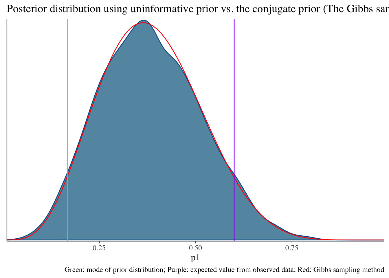
Uninformative prior distribution (2, 6) and posterior distribution
Code
bayesplot::mcmc_dens(fit1$draws('p1')) +geom_path(aes(x = p1, y = pdf), data = pdf_posterior_forplot %>%filter(Alpha_Beta =='(2, 6)'), col ="red") +geom_vline(xintercept =1/6, col ="green") +geom_vline(xintercept =3/5, col ="purple") +labs(title ="Posterior distribution using uninformative prior vs. the conjugate prior (The Gibbs sampler) method", caption ='Green: mode of prior distribution; Purple: expected value from observed data; Red: Gibbs sampling method')
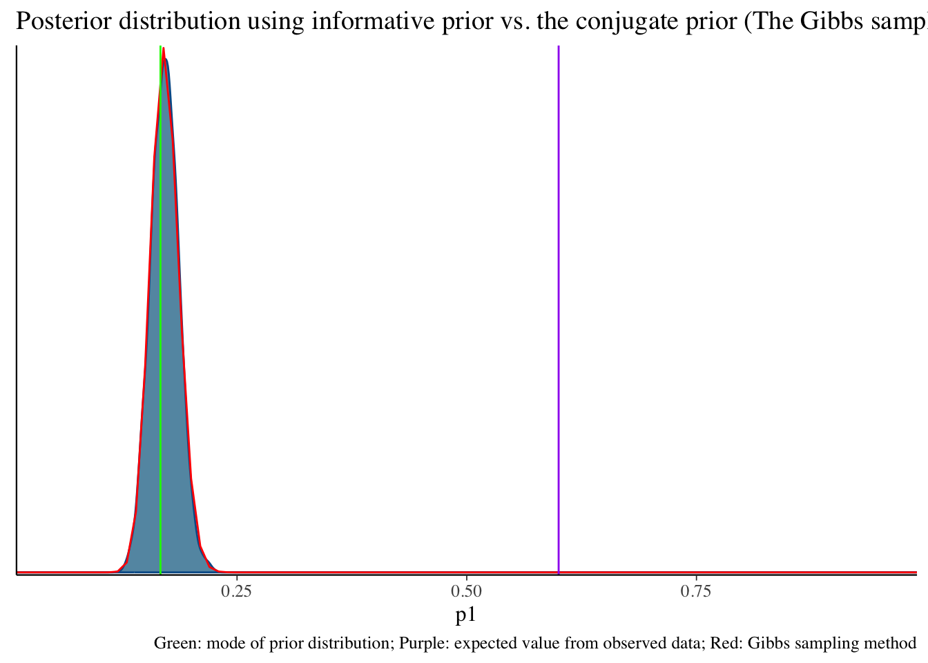
Informative prior distribution (100, 496) and posterior distribution
Code
bayesplot::mcmc_dens(fit2$draws('p1')) +geom_path(aes(x = p1, y = pdf), data = pdf_posterior_forplot %>%filter(Alpha_Beta =='(100, 496)'), col ="red") +geom_vline(xintercept =1/6, col ="green") +geom_vline(xintercept =3/5, col ="purple") +labs(title ="Posterior distribution using informative prior vs. the conjugate prior (The Gibbs sampler) method", caption ='Green: mode of prior distribution; Purple: expected value from observed data; Red: Gibbs sampling method')
Simplifies to: \(\theta^{x + \alpha - 1} (1 - \theta)^{n - x + \beta - 1}\)
This is the kernel of a beta distribution with updated parameters \(\alpha' = x + \alpha\) and \(\beta' = n - x + \beta\). The fact that the posterior is still a beta distribution is what makes the beta distribution a conjugate prior for the binomial likelihood.
Human langauge: Both beta (prior) and binomial (likelihood) are so-called “exponetial family”. The muliplication of them is still a “exponential family” distribution.
Bayesian updating
We can use the posterior distribution as a prior!
1. data {0, 1, 0, 1, 1} with the prior hyperparameter {2, 6} -> posterior parameter {5, 9}
2. new data {1, 1, 1, 1, 1} with the prior hyperparameter {5, 9} -> posterior parameter {10, 9}
3. one more new data {0, 0, 0, 0, 0} with the prior hyperparameter {10, 9} -> posterior parameter {10, 14}
Wrapping up
Today is a quick introduction to Bayesian Concept
Bayes’ Theorem: Fundamental theorem of Bayesian Inference
Prior distribution: What we know about the parameter before seeing the data
hyperparameter: parameter of the prior distribution
Uninformative prior: Prior distribution that does not convey any information about the parameter
Informative prior: Prior distribution that conveys information about the parameter
Conjugate prior: Prior distribution that makes the posterior distribution the same family as the prior distribution
Likelihood: What the data tell us about the parameter
Likelihood function: Probability of the data given the parameter
Likelihood principle: All the information about the data is contained in the likelihood function
Likelihood is a sort of “scientific judgment” on the generation process of the data
Posterior distribution: What we know about the parameter after seeing the data